Bode plots and frequency response
Overview
Only two things can happen to a sine wave passing through a linear, time-invariant system: it's magnitude can be changed; and the signal can be delayed. The delay and percentage change in the magnitude are a function of frequency. A transfer function, H(f), is a complex-valued function of frequency that specifies the magnitude and phase shift of a particular system for all frequencies. The change in amplitude is often called the gain, and the delay is usually thought of in terms of a phase shift of the sine wave.
One way to visualize a transfer function is to make two plots. The first plot shows the gain verses frequency on a set of log-log axes. The second plot shows the phase shift versus log frequency. (Traditionally, Bode plots are constructed only using straight-line segments to represent the transfer function by means of straight edges and fine draft pen sets. Since plotting complicated functions is now done by computer, exact plots may be substituted for the traditional methods.)
Frequency response of common filters
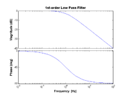
For example, consider a simple RC low-pass filter with the transfer function is given by
- $ H(f) = \frac{V_{out}}{V_{in}} = \frac{1}{1 + j2\pi f RC} $
In this case the cutoff frequency is given by $ f_C = 1 / (2\pi RC) $. Several key features should be noted in the transfer function plot. For frequencies below $ f_C $, the gain is nearly flat (in this case at 1 or 0dB). For frequencies above $ f_C $, the gain drops off by a factor of 10 for each decade in frequency (expressed here in dB as -20dB/decade). At low frequency, the phase starts out at 0°, but starts to decrease noticeably at about $ f_C $/10, drops to −45° at $ f=f_C $, and asymptotes at -90° above 10×$ f_C $.
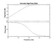
A high-pass filter may be constructed simply by exchanging the R and C components of the low-pass filter. The high-pass filter transfer function is given by
- $ H(f) = \frac{j f / f_{\rm HP}}{1 + j f / f_{\rm HP}} $
where $ f_{\rm HP} $ is the cutoff frequency (the same as before). In this case the gain is 1 only for frequencies $ f>f_{\rm HP} $ and falls off for frequencies below $ f_{\rm HP} $. The phase plot appears identical to the low-pass case, but actually starts at +90° at low frequency and goes to 0° at high frequency.
A second-order low-pass can be constructed by cascading two low-pass filters together in series. Assuming the cutoff frequency of the two filters are the same (and the second stage does not load down the first stage significantly), the transfer function is simply the square of a 1st-order low pass,
- $ H(f) = \left(\frac{1}{1 + j f / f_{\rm LP}}\right)^2 $
This frequency response looks very similar to that of the 1st-order low pass, but the plot scale is double for both gain and phase. The phase again starts out at 0° at low frequency and goes to -1800° at high frequency. For frequencies above $ f_{\rm LP} $, the gain drops off at -40dB/decade. But remember this is a log scale, so the gain attenuates by a factor of 100 at $ f=10f_{\rm LP} $ (and 10000 at $ f=100f_{\rm LP} $). The 2nd-order filter is considerably more effective at filtering out undesirable frequencies.
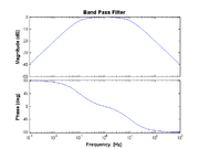
Finally, a band pass can be constructed from appropriately chosen low-pass and high-pass filters in series,
- $ H(f) = \frac{j f / f_{\rm HP}}{1 + j f / f_{\rm HP}} \times \frac{1}{1 + j f / f_{\rm LP}} $
With $ f_{\rm HP}<<f_{\rm LP} $, the gain is 1 (0dB) for frequencies $ f_{\rm HP}<f<f_{\rm LP} $.
MATLAB code
The transfer function plots were generated by the Matlab script wikibodeplots.m.


