Difference between revisions of "Lab Manual: Limits of Detection"
(→Measuring force) |
(→Measuring force) |
||
| Line 50: | Line 50: | ||
==Measuring force== | ==Measuring force== | ||
[[File:Fish-o-meter.png|thumb|right]] | [[File:Fish-o-meter.png|thumb|right]] | ||
| + | Fish are incredibly cool[https://www.youtube.com/watch?v=5SpxY5OLLxc]. Some species, like the ocean sunfish, have pretty comical swimming strokes. For a long time, many people thought that sunfishes were basically at the mercy of the tides. How could a creature with such a silly method of locomotion possibly end up where it wants to be? It turns out that [http://journals.plos.org/plosone/article?id=10.1371/journal.pone.0003446 sunfish are pretty good at going where they want to go.] | ||
| + | |||
| + | Say that you wanted to compare the swimming force generated by the sunfishes' ridiculous motion to, say, the more conventional wriggle of a tuna. One way to measure the the two fishes might be to attach a [[https://en.wikipedia.org/wiki/Spring_scale spring scale]] to an example of each of the fishes and set them on their way. Spring scales exploit Hooke's law, <math>f=-\alpha;x</math>, to measure force. The scale has a zero point marked at the equilibrium position of the spring. Force is indicated by the difference between the length of the spring under tension and the equilibrium length. | ||
==AFM and optical trap model== | ==AFM and optical trap model== | ||
Revision as of 04:33, 28 December 2015
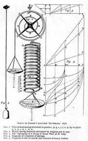
—Robert Hooke (1675)
Ut tensio, sic vis
—Robert Hooke De potential restitutive (1678)
The Power of any Spring is in the same proportion with the Tension thereof: That is, if one power stretch or bend it one space, two will bend it two, and three will bend it three, and so forward. Now as the Theory is very short, so the way of trying it is very easy ... it is very evident that…in every springing body…the force or power thereof to restore it self to its natural position is always proportionate to the Distance or space it is removed therefrom.
—Robert Hooke De potential restitutive (1678)
Overview
Atomic force microscopy and optical trapping are key techniques for investigating forces in biological systems at cellular and molecular levels. Both instruments can exert and measure forces on submicron-scale particles. This capability offers a unique and valuable tool for manipulating and measuring cell components at the single molecule level. For example, optical traps have been used extensively to investigate the mechanical properties of biological polymers and the force generation mechanisms of molecular motors. In many studies, optical tweezers apply force to functionalized microspheres, which act as convenient handles attached to molecules of interest.
To make quantitative force measurements, AFMs and optical traps record displacement of objects being measured versus time. For small displacements, the exerted force is very nearly proportional to displacement. The force/displacement relationship is modeled by Hooke's law: F = -αx, where α is the spring constant. The detector produces a voltage proportional to displacement. The constant of proportionality that converts voltage to distance is called the responsivity of the instrument and denoted by the letter R. Both α and R must be found through a process called calibration. Accurate force and position measurements depend on careful calibration of R and α. On the AFM, α is a function of the cantilever geometry. The optical trap's stiffness depends on trapping laser power, bead size, bead composition, and optical properties of the sample.
In this lab, you will investigate the limits of force detection using AFM and optical traps. You must attend a one-hour lab session during which an instructor will help you take data. You will analyze the data to determine α and R, and you will calculate the minimum detectable force, δ, for both instruments.
Background reading
- Neuman & Nagy. Single-molecule force spectroscopy: optical tweezers, magnetic tweezers and atomic force microscopy. Nature Methods - 5, 491 - 505 (2008).
Measuring force
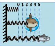
Fish are incredibly cool[1]. Some species, like the ocean sunfish, have pretty comical swimming strokes. For a long time, many people thought that sunfishes were basically at the mercy of the tides. How could a creature with such a silly method of locomotion possibly end up where it wants to be? It turns out that sunfish are pretty good at going where they want to go.
Say that you wanted to compare the swimming force generated by the sunfishes' ridiculous motion to, say, the more conventional wriggle of a tuna. One way to measure the the two fishes might be to attach a [spring scale] to an example of each of the fishes and set them on their way. Spring scales exploit Hooke's law, $ f=-\alpha;x $, to measure force. The scale has a zero point marked at the equilibrium position of the spring. Force is indicated by the difference between the length of the spring under tension and the equilibrium length.
AFM and optical trap model
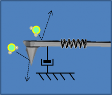
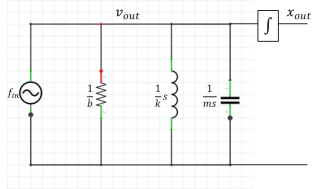
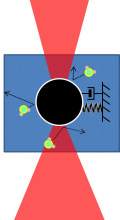
The AFM and the optical trap can both be modeled by a linear system with a mass, spring, and damper in parallel, as shown in the figure below. (The elements all have the same velocity, so they are connected in parallel.) In the AFM, the restoring forceAir or water molecules collide with the cantilever or trapped particle, which drives the system with white noise.
|
|
|
| RLC circuit model of AFM excited by collisions with air molecules. The integrator converts velocity to position. | ||
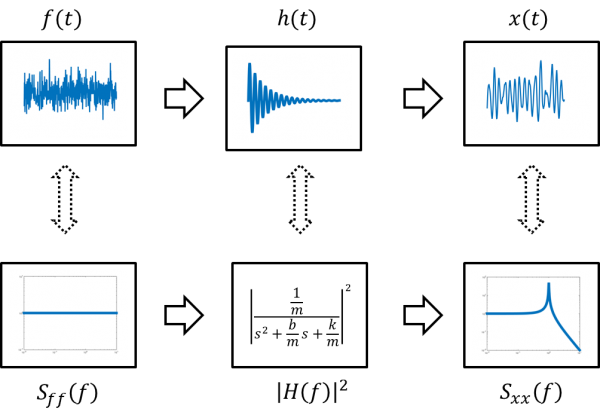
The transfer function of the circuit model is:
- $ \frac{x_{out}}{f_{in}}=\frac{\frac{1}{m}}{s^2+\frac{b}{m}s+\frac{k}{m}} $
In the time domain, random force input $ f(t) $ drives a second-order system to produce position output $ x(t) $.
The driving force has a constant power spectrum $ P_{ff}=\frac{2K_BT}{\pi^2\Beta} $. The output power spectrum $ P_{xx}(f) $ is equal to the input spectrum times the magnitude of the transfer function squared.
Optical trap procedure
The optical trap software produces four columns of tab-delimited data. The first two columns are the X- and Y-QPD voltages. Use the QPD responsivity, R, to convert the QPD voltages to position.The third and fourth columns are the X- and Y-axis sample stage readouts in Volts. To convert the voltage to position, use the responsivity of the stage, Rstage = 2.2 μm/V.
The calibration methods are summarized below:
| Method | Equation | QPD Responsivity | Stage Responsivity | Solvent Viscosity | Particle Diameter | Temperature | Technical Noise |
|---|---|---|---|---|---|---|---|
| $ R_{QPD} $ | $ R_{stage} $ | $ \eta $ | $ d $ | $ T $ | |||
| Equipartition | $ \frac{K_B T}{\langle ^{V_{qpd}}/_{R_{qpd}} \rangle ^ 2} $ | inverse square | none | none | none | linear and indirect (viscosity change) | systematic decrease |
| PSD | $ \left. {6 \pi^2 \eta d \, f_0} \right. $ | none | none | linear | linear | indirect (viscosity change) | small |
| Stokes | $ \langle \frac{3 \pi \eta d \, R_{stage} \, ^{d V_{stage}} / _{dt}} { ^{V_{qpd}}/_{R_{qpd}}} \rangle $ | inverse | linear | linear | linear | indirect (viscosity change) | none |
Report requirements
- Optical trap
- Find R for each power setting by the PSD method.
- Find α for each laser power setting by the Stokes, equipartition, and PSD method.
- Plot R versus laser power for the PSD method.
- Plot α versus laser power for all three methods.
- Calculate $ \delta_x $ and $ \delta_f $ for each laser power setting.
- AFM
- Find the photodiode responsivity R from the calibration data
- Find the lever stiffness k
- How far would the cantilever deflect if you placed a paperclip on the end?
- Calculate $ \delta_z $ and $ \delta_f $ for the AFM cantilever in air

