Assignment 4 part 2: Measure resolution

Overview

Synthetic image of tiny microspheres used for measuring resolution.

This is part 2 of Assignment 4.

One of the most commonly used definitions of resolution is the distance between two point sources in the sample plane such that the peak of one source’s image falls on the first minimum of the other source’s image. The definition suggests a procedure for measuring resolution: make an image of a point source; measure the peak-to-trough distance in the image plane; and divide by the magnification. In this part of the lab, you will use a procedure inspired by this simple idea to estimate the resolution of your microscope. Instead of measuring the spot sizes with a ruler, you will use nonlinear regression on a digital image of point sources.

One practical problem with this method is that true point sources are difficult to come by. If you are using a telescope, stars are readily available to image and they are very good approximations of point sources. Since there is no natural microscopic sample that is equivalent to the night sky, microscopists have to construct something suitable. One of the most common facsimiles is a microscope slide sprinkled with tiny, fluorescent beads that have diameters in the range of 100-190 nm. These beads are small enough to be considered point sources. Unfortunately, beads small enough for this purpose are not very bright. Imaging them can be challenging. Your microscope must be very well aligned to get good results. To measure the spots, you will use nonlinear regression to fit a model curve to the

In this part of the assignment, you will use image processing functions to locate fluorescent microspheres in an image and nonlinear regression to fit a Gaussian function to each bead's image. You will use the best-fit parameters from the regression to determine the resolution measurement.

Why fit a Gaussian instead of a Bessel function? Gaussians are more amenable to nonlinear regression because they are smoother and faster to evaluate than Bessel functions. In addition, the Gaussian is a very good approximation to the central bump of a Bessel function. It is straightforward to convert the Gaussian parameters to Rayleigh resolution. See Converting Gaussian fit to Rayleigh resolution for a discussion of the conversion.

Measuring resolution

The sequence of steps for the resolution code is:

1. find the connected regions and compute properties
2. eliminate connected regions that are likely not image of a single microscphere
3. use nonlinear regression to fit a Gaussian model function to the image of each microsphere
4. compute summary statistics
5. convert Gaussian parameter to Rayleigh resolution

Finding and computing properties of connected regions

There are many methods for segmenting images. Fortunately, the fluorescent images of microspheres you are making in the lab usually have excellent contrast and high SNR. Because of this, a simple, global threshold works well. The Image Processing Toolbox includes several functions that are useful for this purpose.

The function FindBrightObjectsInImage below performs a global threshold and then computes properties of the connected regions of pixels that are above the threshold using the MATLAB Image Processing Toolbox function regionprops. Here is a complete list of the properties regionprops can compute.

function RegionProperties = FindBrightObjectsInImage( ...
        InputImage, GlobalThreshold, DilationRadius, PropertyList )

    mask = im2bw(InputImage, GlobalThreshold);
    mask = imclearborder(mask);               % eliminates connected regions that touch the edge
    mask = imdilate(mask, strel( 'disk', DilationRadius ));  % open up the mask a little
    
    RegionProperties = regionprops( mask, InputImage, PropertyList );

end

FindBrightObjectsInImage returns is a struct array with all of the computed properties —, an array where each element is a structure. There will be one field for each of the properties in the PropertyList argument. The fields have the same name as the property. For example, if you included 'Centroid' in the property list and there were ten objects in the image, RegionProperties(3).Centroid would return a 1 x 2 matrix with the y and x coordinates of the centroid. If you wanted to create a matrix with all of the centroid values, you can use MATLAB's : indexing syntax and a concatenation function: AllCentroids = vertcat( RegionProperties(:).Centroid );.

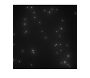
Try running FindBrightObjectsInImage on one of the synthetic images you generated in part 1 and examine the results.

Using nonlinear regression to measure resolution objects

regionprops has no built-in method for measuring resolution, so we will have to write our own. We will use nonlinear regression to compute parameters for each of the PSF bead images.

Regression concepts review

Nonlinear regression is a method for finding the relationship between a dependent quantity $ O_n $ and an one or more independent variables, the spatial coordinates $ x_n $ and $ y_n $ in this case. The variables are related by a model function $ f(\beta, x_n, y_n) $. $ \beta $ is a vector of model parameters. The dependent variable $ y_n $ is measured in the presence of random noise, which is represented mathematically by a random variable $ \epsilon_n $. In equation form:

$ O_n=f(\beta, x_n, y_n)+\epsilon_n $.

The goal of regression is to determine a set of best-fit model parameters $ \hat{\beta} $ that match an observed data as closely as possible. Because the dependent variable includes noise, $ \beta $ cannot be determined exactly from the data. Increasing the number of observations or decreasing the magnitude of the noise tends to produce a more reliable estimate of $ \beta $.

Linear and nonlinear regression are similar in some aspects, but the two techniques have a fundamental difference. Nonlinear regression cannot be reduced to a single, deterministic formula like linear regression. Finding the optimal solution to a nonlinear regression is an iterative process. Nonlinear regression begins with an initial guess. Each iteration produces a more refined estimate of $ \beta $. The process stops when no better estimate can be found (or when something bad happens ... such as the solution not converging).

Ordinary nonlinear least squares regression assumes that:

• the independent variable is known exactly, with zero noise,
• the error values are independent and identically distributed,
• the distribution of the error terms has a mean value of zero,
• the independent variable covers a range adequate to define all the model parameters, and
• the model function exactly relates $ M $ to $ x $ and $ y $.

These assumptions are almost never perfectly met in practice. It is important to consider how badly the regression assumptions have been violated when assessing results.

In the regression we are about to do, the coordinates x and y of each pixel in the image of a PSF bead are known essentially exactly but the measured intensity of each pixel is subject to noise. This makes it easy to determine the best choice of dependent and independent variables. x and y will be the independent variables and the pixel value will be the dependent variable.

Get ready …

You need four things to run a regression:

1. a matrix containing the values of the independent variable(s);
2. a vector containing the corresponding observed values of the dependent variable;
3. a model function; and
4. a vector of initial guesses for the model parameters.

Independent variable and observations

Model function

nlinfit requires that the regression model be expressed as a function that takes two arguments and returns a single vector of predicted values. The signature of the model function must must have the form:

[ PredictedValues ] = ModelFunction( Beta, X ).

The first argument, Beta, is a vector of model parameters. The second argument, X is a vector of independent variable values. The return value, PredictedValues, must must have the same size as X.

The MATLAB function Gaussian2DFitFunction defined below computes the two dimensional function that we will use to model the image of a PSF bead. Parameters is a 1x5 vector that contains the model parameters in this order: X center, Y center, amplitude, sigma, and offset.

function out = Gaussian2DFitFunction( Parameters, Coordinates )
    yCenter = Parameters(1);
    xCenter = Parameters(2);
    amplitude = Parameters(3);
    sigma = Parameters(4);
    offset = Parameters(5);
    
    out = amplitude * ...
        exp( -(( Coordinates(:, 1) - yCenter ).^2 + ( Coordinates(:, 2) - xCenter ).^2 ) ...
        ./ (2 * sigma .^ 2 )) + offset;
    
end

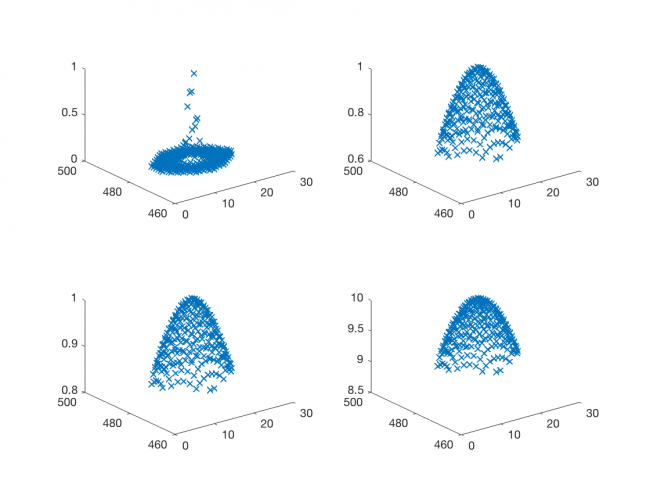
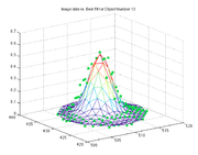
It's a good idea to test the model function out before you use it. The plot below shows four sets of curves generated by Gaussian2DFitFunction . It's comforting to see that the curves have the expected shape.

Initial guesses

nlinfit requires an initial value for each of the three model parameters, contained in a 1x5 vector. (nlinfit infers the number of model parameters from the size of the Initial guess vector.)

    pixelCountAboveHalf = sum( Values > ( ( min( Values ) + max( Values ) ) / 2 ) );
    sigmaInitialGuess = 0.8 * sqrt( pixelCountAboveHalf / 2 / pi / log(2) );

    initialGuesses = [ ...
        mean( Coordinates(:, 1) ), ... % yCenter
        mean( Coordinates(:, 2) ), ... % xCenter
        range( Values ), ... % amplitude
        sigmaInitialGuess, ... % sigma
        min( Values ) ]; % offset

Get set …

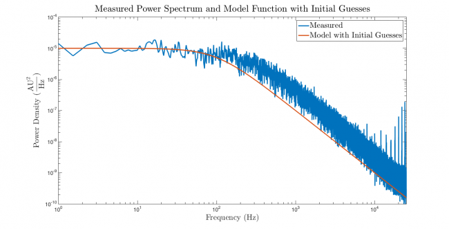
The first step of all regressions is to plot the observations and the model function evaluated with the initial guesses versus the independent variable on a single set of axes. Don't attempt to run nlinfit until you've done this plot. It is much easier to ensure that the arguments to nlinfit are plausible before you invoke it than to debug a screen full of cryptic, red text afterwards. Side effects of premature regression include confusion, waste of time, fatigue, irritability, alopecia, and feelings of frustration. Contact your professor if your regression lasts more than four hours. There is no chance that nlinfit will succeed if there is a problem with one of its arguments.

Go ahead ... do the plot.

Now we can proceed with confidence that the arguments to nlinfit are credible.

Go ... first attempt

Here is a function that puts the whole nonlinear regression process together:

function BestFitParameters = Fit2dGaussian( Values, Coordinates )
    pixelCountAboveHalf = sum( Values > ( ( min( Values ) + max( Values ) ) / 2 ) );
    sigmaInitialGuess = 0.8 * sqrt( pixelCountAboveHalf / 2 / pi / log(2) );

    initialGuesses = [ ...
        mean( Coordinates(:, 1) ), ... % yCenter
        mean( Coordinates(:, 2) ), ... % xCenter
        range( Values ), ... % amplitude
        sigmaInitialGuess, ... % sigma
        min( Values ) ]; % offset

    BestFitParameters = nlinfit( Coordinates, Values, @Gaussian2DFitFunction, initialGuesses );
end

function out = Gaussian2DFitFunction( Parameters, Coordinates )
    yCenter = Parameters(1);
    xCenter = Parameters(2);
    amplitude = Parameters(3);
    sigma = Parameters(4);
    offset = Parameters(5);
    
    out = amplitude * ...
        exp( -(( Coordinates(:, 1) - yCenter ).^2 + ( Coordinates(:, 2) - xCenter ).^2 ) ...
        ./ (2 * sigma .^ 2 )) + offset;
    
end

Before you regress&hellpi;

It's frequently the case that a few of the beads in a real PSF image are not good candidates for measuring resolution. For example, there are sometimes two beads that too close together to separate. Sometimes, there are also aggregates of multiple beads in the picture. Identify some useful properties that region-ropes computes for sorting out the bad regions and write code to eliminate them.

A bit of MATLAB syntax that you might find useful is this: you can remove an element from an array by assigning it to be the empty value []. Some examples:

RegionProperties(3) = []; % removes the third element of the struct array and reduces its size by 1
RegionProperties( [ 0 0 0 1 0 1 0 0 1 0 ] ) = []; % removes the 4th, 6th, and 9th elements and reduces size by 3

Measuring resolution

EstimateResolutionFromPsfImage takes a point-source image and estimates the resolution of an optical system. It uses the built-in MATLAB function im2bw to locate bright regions and regionprops to measure attributes of each connected region of bright pixels. After rejecting outliers, the function uses nlinfit to estimate best fit Gaussian parameters for each bright spot. The optional second argument controls the rejection range for outliers.

There are four subfunctions that should be included in the same m-file as EstimateResolutionFromPsfImage.

function [ Resolution, StandardError, BestFitData ] = MeasureResolutionFromPsfImage( ImageData )

    
    % convert the image to souble precision, if needed
    if ~isa( ImageData, 'double' )
        ImageData = double( ImageData );
    end
    
    % TODO list:
    % 1. think of a good way to pick the threshold
    % 2. figure out how to eliminate images that are not single beads
    
    objectProperties = FindBrightObjectsInImage( ImageData, 0.5, 2, { 'Centroid', 'PixelList', 'PixelValues' } );
    
    labelShift = -9;
    fontSize = 10;
    
    figure
    imshow( ImageData );
    
    for ii = 1:length(objectProperties)
        unweightedCentroid = objectProperties(ii).Centroid;
        text(unweightedCentroid(1) + labelShift, unweightedCentroid(2), ...
            num2str(ii), 'FontSize', fontSize, 'HorizontalAlignment', ...
            'Right', 'Color', [0 1 0]);
    end
    
    % INSERT YOUR CODE TO ELIMINATE BAD OBJECTS HERE

    BestFitData = cell(1, length(objectProperties));
    
    figure;
    
    % use nlinfit to fit a Gaussian to each object
    for ii = 1:length(objectProperties)
        % initial guess for sigma based on area of bright spot
        maximumPixelValue = max( objectProperties(ii).PixelValues );
        darkPixelValue = median( objectProperties(ii).PixelValues );
        pixelCountAboveHalf = sum( objectProperties(ii).PixelValues > .5 *  ( maximumPixelValue + darkPixelValue ) );
        sigmaInitialGuess = 0.8 * sqrt( pixelCountAboveHalf / 2 / pi / log(2) );
        
        initialGuesses = [ ...
            objectProperties(ii).Centroid(1), ... % yCenter
            objectProperties(ii).Centroid(2), ... % xCenter
            max(objectProperties(ii).PixelValues) - min(objectProperties(ii).PixelValues), ... % amplitude
            sigmaInitialGuess, ... % (objectProperties(ii).BoundingBox(3) - 6) / 4, ... % sigma
            min(objectProperties(ii).PixelValues) ];
      
        BestFitData{ii} = nlinfit( objectProperties(ii).PixelList, objectProperties(ii).PixelValues, @Gaussian2DFitFunction, initialGuesses );
        
        % plot data, initial guess, and fit for each peak
        figure(2)
        clf
        
        % generate a triangle mesh from the best fit solution found by 
        % nlinfit and plot it
        gd = delaunay( objectProperties(ii).PixelList(:,1), ...
            objectProperties(ii).PixelList(:,2) );
        trimesh( gd, objectProperties(ii).PixelList(:,1), ...
            objectProperties(ii).PixelList(:,2), ...
            Gaussian2DFitFunction(BestFitData{ii}, ...
            objectProperties(ii).PixelList ) )
        hold on
        
        % plot initial guesses -- commented out to make plots less
        % cluttered. put this back in to debug initial guesses
        % plot3( objectProperties(ii).PixelList(:,1), ...
        %   objectProperties(ii).PixelList(:,2), ...
        %   Gaussian2DFitFunction(initialGuesses, ...
        %   objectProperties(ii).PixelList ), 'rx' )
        
        % plot image data
        plot3( objectProperties(ii).PixelList(:,1), ...
            objectProperties(ii).PixelList(:,2), ...
            objectProperties(ii).PixelValues, 'gx', 'LineWidth', 3)
        title(['Image data vs. Best Fit for Object Number ' num2str(ii)]);
    end
    
    allPeakData = vertcat( BestFitData{:} );
    if( ~isempty( allPeakData ) )
        Resolution = mean( allPeakData(:,4) ) ./ .336;
        StandardError = std( allPeakData(:,4) ./ .336 ) ./ sqrt( length( BestFitData ) );
    else
        Resolution = NaN;
        StandardError = NaN;
    end
end

function out = Gaussian2DFitFunction( Parameters, Coordinates )
    yCenter = Parameters(1);
    xCenter = Parameters(2);
    amplitude = Parameters(3);
    sigma = Parameters(4);
    offset = Parameters(5);
    
    out = amplitude * ...
        exp( -(( Coordinates(:, 1) - yCenter ).^2 + ( Coordinates(:, 2) - xCenter ).^2 ) ...
        ./ (2 * sigma .^ 2 )) + offset;
    
end

Testing the code

Example image processing on PSF beads to determine microscope resolution.

Example Gaussian fit of a PSF bead fluorescence emission profile to estimate microscope resolution.

Use the synthetic image code you developed in part 1 of this assignment to test the EstimateResolutionFromPsfImage function using synthetic images of 170 nm fluorescent microspheres over a range of numerical apertures from 0.1 to 1.0. Plot the results, actual resolution versus measured resolution. Turn in your code and the plot.

Measure the resolution of your microscope

1. Make an image of a sample of 170 nm fluorescent beads with the 40X objective. (Several dozens to hundreds of PSF spheres should be captured in your image.)
   • Use 12-bit mode on the camera and make sure to save the image in a format that preserves all 12 bits.
   • Ensure that the image is exposed properly.
     • Over-exposed images will give inaccurate results.
     • Under-exposed images will be difficult to process and yield noisy results.
   • This procedure is extremely sensitive to the focus adjustment.
   • To minimize photobleaching, do not expose of the beads to the light source and longer than necessary.
   • Be sure to save the image and the histogram for your lab report.
2. Use image processing functions to locate non-overlapping, single beads in the image.
3. Use nonlinear regression to fit a Gaussian to each bead image.
4. Convert the Gaussian parameters to resolution.
   • This page has example MATLAB code.

Report the resolution you measured and discuss sources of error in the measurement.

Back to 20.309 Main Page
Back to Assignment 4 Overview
Back to Assignment 4 Part 1
On to Assignment 4 Part 3