Difference between revisions of "Assignment 4 part 2: Measure resolution"

Overview

In this part of the assignment, you will measure the resolution of your microscope using image processing code that you will develop.

This is part 2 of Assignment 4.

Measuring resolution

One of the most commonly used definitions of resolution is the distance between two point sources in the sample plane such that the peak of one source’s image falls on the first minimum of the other source’s image. The definition suggests a procedure for measuring resolution: make an image of a point source; measure the peak-to-trough distance in the image plane; and divide by the magnification. In this part of the lab, you will use a procedure inspired by this simple idea to estimate the resolution of your microscope. Instead of measuring the spot sizes with a ruler, you will use nonlinear regression on a digital image of point sources.

One practical problem with this method is that true point sources are difficult to come by. If you are using a telescope, stars are readily available to image and they are very good approximations of point sources. Since there is no natural microscopic sample that is equivalent to the night sky, microscopists have to construct something suitable. One of the most common facsimiles is a microscope slide sprinkled with tiny, fluorescent beads that have diameters in the range of 100-190 nm. These beads are small enough to be considered point sources. Unfortunately, beads small enough for this purpose are not very bright. Imaging them can be challenging. Your microscope must be very well aligned to get good results. To measure the spots, you will use nonlinear regression to fit a model curve to the

In this part of the assignment, you will use image processing functions to locate fluorescent microspheres in an image and fit a Gaussian function to them. Why not use a Bessel function? Gaussians are more amenable to nonlinear regression than Bessel functions, and they are a very good approximation. It is straightforward to convert the Gaussian parameters to Rayleigh resolution. See Converting Gaussian fit to Rayleigh resolution for a discussion of the conversion.

Measuring resolution

The sequence of steps for the resolution code is:

1. find the connected regions
2. eliminate connected regions that are likely not image of a single microscphere
3. use nonlinear regression to fit a Gaussian model function to the image
4. compute summary statistics
5. convert Gaussian parameter to Rayleigh resolution

Step 1: find the connected regions

There are many methods for segmenting images. Fortunately, the fluorescent images of microspheres you are making in the lab usually have excellent contrast and high SNR. Because of this, a simple, global threshold works well. The interesting things are the bright ones. The only challenge is where to set the threshold. The Image Processing Toolbox includes several functions that are useful for this purpose.

The function FindBrightObjectsInImage below performs a global threshold and then computes properties of the connected regions of pixels that are above the threshold using the MATLAB Image Processing Toolbox function regionprops. Here is a complete list of the properties regionprops can compute.

function RegionProperties = FindBrightObjectsInImage( InputImage, GlobalThreshold, DilationRadius, PropertyList )

    mask = im2bw(InputImage, GlobalThreshold);
    mask = imclearborder(mask);               % eliminates connected regions that touch the edge
    mask = imdilate(mask, strel( 'disk', DilationRadius ));  % open up the mask a little
    
    RegionProperties = regionprops( mask, InputImage, PropertyList );

end

RegionProperties is an array of structs. A struct or structure is a variable type that aggregates related pieces of data in fields. Each of the fields can be a different data type or size. You can create an array of structs like this:

bar(3) = struct(); % stupid MATLAB syntax for creating a struct array
bar(1).Name = 'Felix';
bar(1).Age = 5;
bar(1).Species = 'Cat'
bar(1).Weight = 6;
bar(2).Name = 'Spot';
bar(2).Age = 2;
bar(2).Species = 'Dog'
bar(2).Weight = 18;
bar(3).Name = 'Tony';
bar(3).Age = 30;
bar(3).Species = 'Tiger'
bar(3).Weight = 40;

So bar(2).Age returns 2, and bar(3).Name returns 'Tony'. If you wanted a column vector that contained the age field of all the elements, you can generate that with: vertcat( bar(:).Age );.

Measuring resolution

The sequence of steps for processing is

EstimateResolutionFromPsfImage takes a point-source image and estimates the resolution of an optical system. It uses the built-in MATLAB function im2bw to locate bright regions and regionprops to measure attributes of each connected region of bright pixels. After rejecting outliers, the function uses nlinfit to estimate best fit Gaussian parameters for each bright spot. The optional second argument controls the rejection range for outliers.

There are four subfunctions that should be included in the same m-file as EstimateResolutionFromPsfImage.

function [ Resolution, StandardError, BestFitData ] = MeasureResolutionFromPsfImage( ImageData )

    
    % convert the image to souble precision, if needed
    if ~isa( ImageData, 'double' )
        ImageData = double( ImageData );
    end
    
    % TODO list:
    % 1. think of a good way to pick the threshold
    % 2. figure out how to eliminate images that are not single beads
    
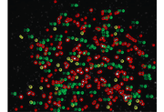
    objectProperties = FindBrightObjectsInImage( ImageData, 0.5, 2, { 'Centroid', 'PixelList', 'PixelValues' } );
    
    labelShift = -9;
    fontSize = 10;
    
    figure
    imshow( ImageData );
    
    for ii = 1:length(objectProperties)
        unweightedCentroid = objectProperties(ii).Centroid;
        text(unweightedCentroid(1) + labelShift, unweightedCentroid(2), ...
            num2str(ii), 'FontSize', fontSize, 'HorizontalAlignment', ...
            'Right', 'Color', [0 1 0]);
    end
    
    % INSERT YOUR CODE TO ELIMINATE BAD OBJECTS HERE

    BestFitData = cell(1, length(objectProperties));
    
    figure;
    
    % use nlinfit to fit a Gaussian to each object
    for ii = 1:length(objectProperties)
        % initial guess for sigma based on area of bright spot
        maximumPixelValue = max( objectProperties(ii).PixelValues );
        darkPixelValue = median( objectProperties(ii).PixelValues );
        pixelCountAboveHalf = sum( objectProperties(ii).PixelValues > .5 *  ( maximumPixelValue + darkPixelValue ) );
        sigmaInitialGuess = 0.8 * sqrt( pixelCountAboveHalf / 2 / pi / log(2) );
        
        initialGuesses = [ ...
            objectProperties(ii).Centroid(1), ... % yCenter
            objectProperties(ii).Centroid(2), ... % xCenter
            max(objectProperties(ii).PixelValues) - min(objectProperties(ii).PixelValues), ... % amplitude
            sigmaInitialGuess, ... % (objectProperties(ii).BoundingBox(3) - 6) / 4, ... % sigma
            min(objectProperties(ii).PixelValues) ];
      
        BestFitData{ii} = nlinfit( objectProperties(ii).PixelList, objectProperties(ii).PixelValues, @Gaussian2DFitFunction, initialGuesses );
        
        % plot data, initial guess, and fit for each peak
        figure(2)
        clf
        
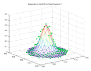
        % generate a triangle mesh from the best fit solution found by 
        % nlinfit and plot it
        gd = delaunay( objectProperties(ii).PixelList(:,1), ...
            objectProperties(ii).PixelList(:,2) );
        trimesh( gd, objectProperties(ii).PixelList(:,1), ...
            objectProperties(ii).PixelList(:,2), ...
            Gaussian2DFitFunction(BestFitData{ii}, ...
            objectProperties(ii).PixelList ) )
        hold on
        
        % plot initial guesses -- commented out to make plots less
        % cluttered. put this back in to debug initial guesses
        % plot3( objectProperties(ii).PixelList(:,1), ...
        %   objectProperties(ii).PixelList(:,2), ...
        %   Gaussian2DFitFunction(initialGuesses, ...
        %   objectProperties(ii).PixelList ), 'rx' )
        
        % plot image data
        plot3( objectProperties(ii).PixelList(:,1), ...
            objectProperties(ii).PixelList(:,2), ...
            objectProperties(ii).PixelValues, 'gx', 'LineWidth', 3)
        title(['Image data vs. Best Fit for Object Number ' num2str(ii)]);
    end
    
    allPeakData = vertcat( BestFitData{:} );
    if( ~isempty( allPeakData ) )
        Resolution = mean( allPeakData(:,4) ) ./ .336;
        StandardError = std( allPeakData(:,4) ./ .336 ) ./ sqrt( length( BestFitData ) );
    else
        Resolution = NaN;
        StandardError = NaN;
    end
end

function out = Gaussian2DFitFunction( Parameters, Coordinates )
    yCenter = Parameters(1);
    xCenter = Parameters(2);
    amplitude = Parameters(3);
    sigma = Parameters(4);
    offset = Parameters(5);
    
    out = amplitude * ...
        exp( -(( Coordinates(:, 1) - yCenter ).^2 + ( Coordinates(:, 2) - xCenter ).^2 ) ...
        ./ (2 * sigma .^ 2 )) + offset;
    
end

Testing the code

Use the synthetic image code you developed in part 1 of this assignment to test the EstimateResolutionFromPsfImage function using synthetic images of 170 nm fluorescent microspheres over a range of numerical apertures from 0.1 to 1.0. Plot the results, actual resolution versus measured resolution. Turn in your code and the plot.

Measure the resolution of your microscope

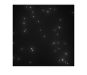
1. Make an image of a sample of 170 nm fluorescent beads with the 40X objective. (Several dozens to hundreds of PSF spheres should be captured in your image.)
   • Use 12-bit mode on the camera and make sure to save the image in a format that preserves all 12 bits.
   • Ensure that the image is exposed properly.
     • Over-exposed images will give inaccurate results.
     • Under-exposed images will be difficult to process and yield noisy results.
   • This procedure is extremely sensitive to the focus adjustment.
   • To minimize photobleaching, do not expose of the beads to the light source and longer than necessary.
   • Be sure to save the image and the histogram for your lab report.
2. Use image processing functions to locate non-overlapping, single beads in the image.
3. Use nonlinear regression to fit a Gaussian to each bead image.
4. Convert the Gaussian parameters to resolution.
   • This page has example MATLAB code.

Report the resolution you measured and discuss sources of error in the measurement.

Back to 20.309 Main Page
Back to Assignment 4 Overview
Back to Assignment 4 Part 1
On to Assignment 4 Part 3