Difference between revisions of "20.109(S17):Complete cell survival assay and examine transcript levels in response to DNA damage (Day 4)"

Introduction

Today you will be completing two experiments for module 2. The cell viability assay will provide information concerning the conditional lethality of compound 401 (NHEJ inhibitor) and olaparib (PARP inhibitor). In addition, you will use quantitative PCR to assess the levels of specific transcripts in response to DNA damage.

Cell viability assay
The CellTiter-Glo Luminescent Cell Viability Assay is a method for quantifying the number of viable cells based on measuring the amount of ATP present. ATP is a proxy for the presence of metabolically active (alive) cells. In this assay, the cells are lysed and ATP is released from the active cells. In a reaction catalyzed by a propriety luciferase enzyme, luciferin, ATP, and oxygen result in oxyluciferin, AMP, PP_i, carbon dioxide, and light. The light product is then measured using a luminometer.

Quantitative PCR
Quantitative polymerase chain reaction (qPCR) allows researchers to monitor the results of PCR as amplification is occurring (this technique is also referred to as real-time reverse transcription-polymerase chain reaction or real-time PCR). During qPCR data are collected throughout the amplification process using a fluorescent dye. The fluorescent dye is highly specific for double-stranded DNA and when bound to DNA molecules the fluorescence intensity increases proportionately to the increase in double-stranded product. In contrast, the data for traditional PCR are simply observed as a band on a gel.

As depicted in the image to the right, the fluorescent dye binds to double-stranded DNA during the cycles of PCR. At the annealing temperature the primer (blue arrow) binds to the template (black line). During an incubation at the extension temperature the new copy of DNA (orange dashed arrow) is sythesized by the polymerase enzyme. The inactive fluorescent dye molecules present in the reaction (grey stars) bind to the newly generated double-stranded DNA and become activated (green stars).

To assess gene transcript levels, you will examine the C_T values from your qPCR assay. The C_T values are displayed as an amplification curve following qPCR (these values are also given numerically). The initial cycles measure very little fluorescence due to low amounts of double-stranded DNA and are used to establish the inherent background fluorescence. As double-stranded product is produced, fluorescence is measured and the curve appears linear. This linear portion of the curve represents the exponential phase of PCR. Throughout the exponential phase, the curve should be smooth. Sharp points may be due to errors in reaction preparation or failures in the machine used to measure fluorescence. As mentioned previously, the first cycle in which the fluorescence measurement is above background is the C_T. During the later cycles the curve shows minimal increases in fluorescence due the depletion of reagents.

Following the qPCR amplification measurements, a melt curve is completed. Melt curves assess the dissociation of double-stranded DNA while the sample is heated. As the temperature is increased, double-stranded DNA ‘melts’ as the strands dissociate. As discussed above, the fluorescent dye used in qPCR associates with double-stranded DNA and fluorescence measurements will decrease as the temperature increases. In qPCR, the melt curve is used to confirm that a single amplification product was generated during the reaction. If additional products were present, the melt curve would presumably show additional peaks. Why might this be true? Can you think of a scenario where two different products would produce a single peak in a melt curve?

Protocols

Part 1: Complete cell viability assay

Today you will complete the second experiment for Mod 2 - the cell viability assay. In the previous class you used etoposide to induce DNA damage and added a NHEJ inhibitor. In addition, you treated your cells with a PARP inhibitor. By comparing the results of these treatments between the DLD-1 and BRCA2- cell lines you will more deeply examine the DNA repair pathways from lecture.

1. Retrieve your plate from the 37 °C incubator.
2. Aspirate the spent media from each well.
   • Be careful not to cross-contaminate between the wells.
3. Add 500 μL of fresh media into each well.
   • You should also add media to the well that was empty as this will be your background control sample.
4. Obtain an aliquot of the CellTiter Glo reagent from the front laboratory bench.
5. Thoroughly mix the CellTiter Glo reagent, then add 500 μL into each well of your plate.
   • After adding the reagent, pipet up and down two times to mix.
6. Move your plate to the plate shaker at the front laboratory bench and shake for 2 min.
7. Remove your plate from the plate shaker and incubate on your benchtop for 10 min.
8. Transfer 100 μL from each well into a white 96-well plate.
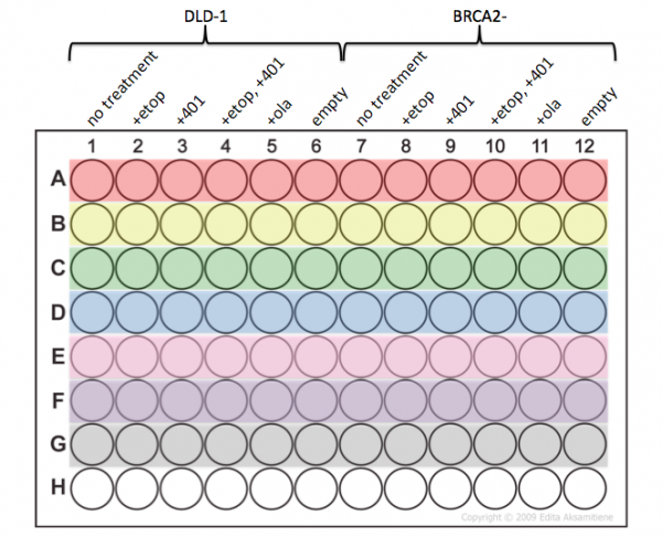
   • Be very careful that you add your samples to the appropriate wells according the plate map below.
     

     

The teaching faculty will take the plate to the BioMicro Center to measure the luminescence from your samples using the Varioskan plate reader.

Part 2: Design quantitative PCR primers

Part 3: Setup quantitative PCR assay

In the previous laboratory session you purified RNA from your DLD-1 and BRCA2- cells and used the RNA to generate cDNA. Today you will use quantitative PCR to probe the transcription levels of genes of interest. Specifically, you will examine the response of DNA damage indicators to evaluate the etoposide treatment. In addition, you will ensure that exon 11 of BRCA2- is not expressed in the null mutant cell line...and that it is expressed in the parental cell line.

Part 3a: Clean cDNA

1. Retrieve your cDNA samples from the front laboratory bench.
2. Add 100 μL of Buffer PB to each cDNA preparation.
3. Place four QIAquick columns into collection tubes and carefully label each according to your cDNA samples.
4. Transfer the entire volume of cDNA + Buffer PB (~120 μL) from each tube into the appropriate QIAquick column.
5. Centrifuge at maximum speed for 30 sec, then discard the flow-through.
6. Add 750 μL of Buffer PE to the QIAquick columns, centrifuge at maximum speed for 30 sec, then discard the flow-through.
7. Centrifuge the QIAquick columns at maximum speed for 1 min.
   • This will remove any residual liquid from the columns.
8. Move each QIAquick column into a clean, labeled 1.5 mL centrifuge tube.
   • Be sure to remove the caps so they do not break off in the centrifuge.
9. Te elute the DNA, add 50 μL of dH₂O pH = 8 to the center of the column and leave at your benchtop for 1 min.
10. Centrifuge at maximum speed for 1 min.
    • The liquid in the microcentrifuge tube is your cleaned cDNA.
11. Alert the teaching faculty when you have finished and you will be escorted to the nanodrop to measure the concentration of your cDNA samples.

Part 3b: Prepare cDNA for quantitative PCR assay

1. Obtain XX PCR tubes from the front laboratory bench and label according to the sample code.
   • A=
2. Using the concentration measurements from Part 3a, calculate the volume of each sample that contains 10 ng of cDNA.
   • If the volume is greater than 7 μL alert the teaching faculty.
3. Prepare master mixes of your samples such that:
   • Each reaction should contain 10 ng of cDNA, 3 μL of the appropriate diluted primer solution, and water for a total volume of 10 μL.
   • The volume of water is calculated as 7 μL minus the volume calculated in Step #2 for each sample.
   • For each sample/primer set combination, prepare enough for 3.5 reactions.
4. Add your reactions to the plate on the front bench according to the map. You will add 12.5 μL to each well.
5. Once everyone has added their reactions, the teaching faculty will add 10 μL of the 2X Syber Green master mix to each well.

For your reference, the PCR cycling conditions are listed below:

Stage	Cycles	Details
1	1	95°C for 10 min
2	40	95°C for 15 sec 60°C for 30 sec 72°C for 30 sec
3	1	4°C hold

Reagents

• CellTiter Glo cell viability assay kit (Promega)

Navigation links

Next day: Journal club I

Previous day: Purify RNA for quantitative PCR assay and treat cells for survival assay