20.109(S20):Analyze SMM data (Day6)

Introduction

Today is the culminating day of Module 1! Hopefully you will identify 'hits' from your SMM screen, or ligands that are able to bind TDP43-RRM12. Though you may be able to qualitatively visualize spots that appear to emit more fluorescence, it is important to complete quantitative analysis that supports your observations.

During our previous laboratory session, you used microarrayer to read the fluorescence signals on the surface of the SMM at two excitation wavelengths. As noted previously, the 532 nm wavelength was used to excite fluorescein, which was printed in an 'X' pattern to assist with alignment. The 635 nm wavelength was used to excite the fluorophore-conjugated TDP43-RRM12. A hit denotes a spot on the slide that emits a red fluorescence signal significantly higher than the background fluorescence level. In terms of protein binding, a hit denotes that the TDP43-RRM12 protein is bound to a compound is therefore localized to that position on the slide. You will analyze the fluorescence emission data collected by the microarray scanner using a value termed the robust z-score.

When the Koehler Lab prepared each printed glass slide, the microarrayer also produced a GAL file, or GenePix Array List. The GAL file contains information about where each spot was printed, and what compound was printed there. However, the relationship between the GAL file and the actual contact of the print head is very imprecise. Instead, we will use the fluorescein guide spots to align the array in the GAL file to the true print location for each pin. Following the alignment, we will compare the fluorescence at 635nm within the deposition region of each spot (foreground) to the fluorescence immediately outside of this region, where nothing was printed (background). We’ll use these values to calculate a robust z-score. From the robust z-score, we can determine the associated probability that the observed fluorescence occurred by chance, and if this probability is sufficiently low, we call the compound a hit.

Protocols

Part 1: BE Communication Lab workshop

Our communication instructors, Dr. Sean Clarke and Dr. Prerna Bhargava, will join us today for a workshop on crafting clear and informative figures with captions.

Part 2: Identify hits from SMM results

To complete the data analysis steps outlined in the Prelab discussion and above in the Introduction, you will use a Jupyter notebook generated by Rob Wilson, a graduate student in the Koehler Laboratory. Though the code is provided to you, it is important to critically think through the data analysis steps!

You will work with your partner to complete the data analysis using a laboratory computer (one computer per team!).

1. Open a terminal using the icon in the toolbar.
2. Type "conda activate 20109_SMM" and press the enter key.
   • This command indicates which Python environment should be used.
3. Type "jupyter notebook" and press the enter key.
   • This command opens Jupyter.
4. The Jupyter notebook directory should open in a new window.
5. To select the Jupyter notebook location, select 'Desktop', select '20200221_TDP43-Screen', then select the notebook '20109_S20_SMM_Analysis.ipynb.
6. The notebook should look like the image below:
   

   
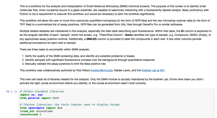
7. The text provides details on what the code below (in boxes) is accomplishing. As you work through the data analysis, make notes in your laboratory notebook regarding the steps completed. Specifically, include the purpose for each step. You will also generate several figures as you complete the analysis, these should also be included in your laboratory notebook with some description of what is shown.

Navigation links

Next day: Examine TDP43 binders for chemical features

Previous day: Scan SMM slides to identify binders of TDP43 protein