Lab Manual: Atomic Force Microscopy (AFM)
Experiment 1: AFM mini-lab
- Read The 20.309 AFM system and Experiment 1: Mini-lab: Measuring Boltzmann's Constant.
- Work with a TA or Instructor.
- Learn the signal paths and connections of the system.
- Practice aligning the AFM optics.
- Learn how to calibrate the AFM to extract useful physical data.
- Measure the vibrational noise floor in the AFM system.
- Use the AFM to record the vibrational noise spectrum of a cantilever probe
Experiment 2: Imaging
- Image several different samples with the AFM and measure physical dimensions of imaged features.
Experiment 3: Elastic modulus
- Use the AFM to measure the elastic modulus and surface adhesion force of several different samples.
The 20.309 AFM System
This section describes the various components of the AFM you will use in the lab, and particularly how they differ in operation from a commercial AFM. In lecture we will discuss the operational principles of a commercial AFM. You may also find it helpful to review some of the references at the end of this module.
Hardware
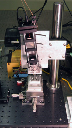
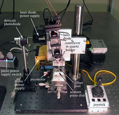
A photo of our AFM setup is provided in Figure 1 for you to refer to as you learn about the instrument. Start by physically examining the setup and identifying all the parts described below.
Motion control system
To be useful for imaging, an AFM needs to scan its probe over the sample surface. Our microscopes are designed with a fixed probe and a movable sample (also true of some commercial AFM systems). Whenever we talk about moving the tip relative to the sample, in 20.309 we will always only move the sample. The sample is actuated for scanning and force spectroscopy measurements by a simple piezo disk, shown in Figure 2. The piezo disk is controlled from the matlab scanning software, which is described in Software.
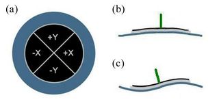
For vertical motion along the z-axis, there are two regimes of motion:
- Manual (coarse): Turning the knob on the knob on the stage clockwise moves the stage up.
- Piezo-disk (fine): Actuating the piezo disk over a few hundred nanometers using the matlab software. For x- and y-axis positioning (in the sample plane), coarse movements are accomplished with the stage micrometers, and fine (several nm) movements are also attained using the piezo disk.
Optical system
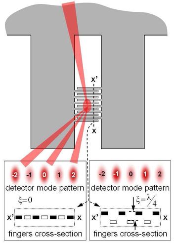
Our microscopes use a somewhat different optical readout from a standard AFM to sense cantilever deflection. Rather than detecting the position of a laser beam that reflects off the back surface of the cantilever, we measure the intensity of a diffracted beam. To do this, a diode laser with wavelength $ \lambda $ = 635 nm is focused onto the interdigitated (ID) finger structure, and we observe the brightness of one of the reflected spots (referred to as "modes") using a photodiode. This gives us information about the displacement of one set of fingers relative to the other — this is useful if one set is attached to the cantilever and the other to some reference surface.
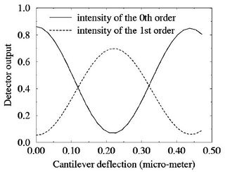
As the cantilever deflects, and the out-of-plane spacing between the ID fingers changes, the reflected diffractive modes change their brightness, as shown in Figure 3. However, a complication of using this system is the non-linear output characteristic of the mode intensities. As the out-of-plane deflection of the fingers increases, each mode grows alternately brighter and dimmer. The intensity $ I $ of odd order modes vs. finger deflection $ \Delta $z has the form
<Leftequation id="eqn:eq1">$ I \propto sin^2 \left( \frac{2\pi}{\lambda}\Delta z \right) $,</Leftequation>
and for odd modes, the sine is replaced by a cosine. The plot in Figure 4a shows graphically the intensity of two adjacent modes as a function of displacement.
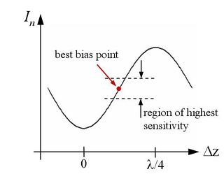
This nonlinearity makes the sensor's sensitivity depend critically on the operating point along this curve at which a measurement is done. To make useful measurements, the ID interferometer therefore needs to be biased to a spot on the $ sin^2 $ curve where the function's slope is greatest midway between the maximum and minimum, as sketched in Figure 4b.
Due to residual strain in the silicon nitride from which the cantilevers are fabricated, the relative planar alignment of the two finger sets varies slightly over the area of the grating. This variation is typically a few hundred nanometers in the lateral direction. Therefore, the bias point of the detector's output can be adjusted along the $ sin^2 $ curve by moving the incident laser spot side to side on the diffraction grating.
| (a) Output of the ID diffractive transducer. The non-linear intensities of the 0th and 1st order modes as a function of cantilever displacement (from Yaralioglu, et al., J. Appl. Phys., 1998), and (b) the desired operating point for maximum deflection sensitivity.
| |
Cantilever probes for imaging
A few words about probe breakage: you will break at least a few probes — this is a normal part of learning to use the tool. We have a large, but not infinite supply of replacement probes. The cost of an individual AFM probe is not large, and the greater problem with breaking them is the time lost to replacing the probe and realigning the laser.
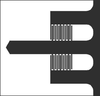
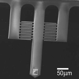
| (a) Plan view of the imaging cantilever geometry, and (b) SEM image of the imaging cantilever. The central (imaging) beam dimensions are length L = 400 μm, and width b = 60 μm. The finger gratings begin 117 μm and end 200 μm from the base.
| |
Exercise caution when moving the sample up and down, but don't let this prevent you from getting comfortable moving the sample around. Under most conditions, the cantilevers are surprisingly flexible and robust. They are most often broken by running them into the sample (especially sideways) — avoid "crashing" the tip into the surface, or worse bumping the stage into the die or fluid cell. Make sure you're familiar with the Motion control system.
The probes we use for imaging are shown in Figure 5 with relevant dimensions. The central beam has a tip at its end, which scans the surface. The shorter side beams to either side have no tips and remain out of contact. The side beams provide a reference against which the deflection of the central beam is measured; the ID grating on either side may be used. When calibrating the detector output to relate voltage to tip deflection, remember to include a correction factor to account for the ID finger position far away from the tip.
Cantilevers for thermal noise measurements
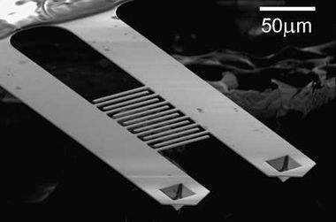
For noise measurement purposes, we'd like a clean vibrational noise spectrum, which is best achieved using a matched pair of identical cantilevers. The configuration with a central long beam and reference side-beams has extra resonance peaks in the spectrum that make it harder to interpret. With the geometry shown in Figure 6 the beams have identical spectra which overlap and reinforce each other. Using a pair of identical beams also helps to minimize any common drift effects from air movements or thermal gradients.
(a) Plan view and (b) SEM image of the geometry of a differential cantilever pair. Because the beams are fabricated so close together, we assume that their material properties and dimensions are identical.
| |
There are two sizes of cantilever pairs available. For the long devices, L = 350 $ \mu $m and the finger grating starts 140 $ \mu $m and ends 250 $ \mu $m from the cantilever base. For the short devices, L = 275 $ \mu $m, and the finger gratings begin 93 $ \mu $m and end 175 $ \mu $m from the base. The width and thickness of all of the cantilevers is b = 50 $ \mu $m and h = 0.8 $ \mu $m, respectively.
Major operational steps
Power-on
For our AFMs to run, you must turn on three things: (1) the detection laser, (2) the photodetector, and (3) piezo-driver power supply. The photodetector has a battery that provides reverse bias, and the others have dedicated power supplies (refer to Figure 1 for where these switches are located). When you finish using the AFM, don't forget to turn off the three switches you turned on at the beginning.
Signal connections and data flow
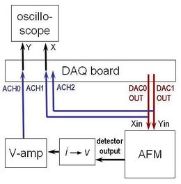
The first key step to using the instrument is properly connecting all of the components together. Figure 7 will help to guide you. The AFM itself requires two signal inputs (Xin and Yin) to drive the piezo actuator, which connect to the electronics board on the back of the headplate. They are provided by the computer's analog signal outputs (NI-USB6212 DAQ channels AO0 and AO1, respectively). The computer also needs to read these two signals in, together with the AFM signal output, so these become the three DAQ inputs, AI1, AI2, and AI0, respectively.
The output from the AFM's photodetector is a current signal, proportional to the brightness of the laser spot, that needs to be converted to a voltage (a 100 k$ \Omega $ resistor to ground is sufficient). It's good to be able to amplify and offset this voltage at our convenience, so we run this signal through a Tektronix AM502 amplifier before it enters the DAQ.
Finally, during calibration, it's very useful to watch the detector signal as a function of stage movement in realtime, on the oscilloscope screen, so we run those signals to the scope as well.
Laser alignment and diffractive modes
To get a cantilever position readout, the laser needs to be well focused on the interdigitated fingers of the cantilever. Use the white light source and stereo-microscope to look at the cantilever in its holder. The laser spot should be visible as a red dot (there may be other reflections or scattered laser light, but the spot itself is a small bright dot). Adjust its position using the knobs on the kinematic laser mount, until it hits the interdigitated fingers (use the cantilever schematics in Figure 5 and Figure 6 as a reference).
When the laser is focused in approximately the right position, the white "screen" around the slit on the photodetector will allow you to see the diffraction pattern coming out of the beam splitter. Observe the spot pattern on this screen while adjusting the laser position until you see several evenly spaced "modes." Make sure you aren't misled by reflections from other parts of the apparatus — some may look similar to the diffraction pattern, but aren't what you're looking for.
When you see the proper diffraction pattern is on the detector, adjust the detector's position such that only one mode passes through the slit. Typically the 0th mode gives the largest difference between bright and dark.
Engaging the tip
The process of bringing the probe tip to the sample surface so we can scan images and measure forces is called "engaging." The aim is to get the tip in close proximity so it is just barely coming into contact, and bending only slightly. If the probe does not touch the surface, it is obviously useless, but if it's bent too much against the surface it can damage the sample or simply push through soft features and report topologies lower than actual.
Before engaging, start the piezo z-modulation scan in the matlab software (see Z-mod (force spectroscopy) operation). Be sure the mode switch on the AFM electronics board is flipped down to "force spec. mode," and make sure to turn on the piezo power supply. Carefully bring the tip near the surface using the stage micrometer for vertical motion. When you make contact, you will see the modes on the photodetector fluctuate in brightness. Because of the device geometry, only the central long cantilever with the tip will make contact with the sample surface.
Calibration and biasing
At this point, it's worth pausing to review the definition of calibration, as well as the distinction between sensitivity and resolution — terms which will often be used frequently in this context, but whose accurate meaning isn't always made explicit. Be sure you're clear on the differences between them.
Calibration is finding the relationship between the output of your instrument to the physical quantity you are measuring like distance or force. In our case, relating the mode brightness measured by the photodiode to cantilever tip deflections.
Sensitivity is a numerical expression for the calibration; e.g., the "slope" of a transducer output in mV/N, W/ºA, or in our case nm/V; i.e., nm of tip deflection versus photodiode voltage. Be careful not to get confused between photodiode voltage and piezo voltage during your calibration step. Also, be sure to accurately account for your gain setting on the AM502.
Resolution is the minimal change in signal that the instrument can detect. It depends completely on the noise, frequency, and bandwidth of the measurement
Calibration
It is essential to run a calibration before performing any measurement because the sensitivity varies from AFM to AFM and user to user. We calibrate our AFM in force spectroscopy (or z-mod) mode, where the sample is only moved straight up and down. In all that follows, it is assumed that the spot is correctly focused (in the z-direction) on the fingers as noted earlier. The goal of this calibration process is to relate the detector's voltage signal to physical tip deflection; in other words, how many nm is the cantilever tip bending for every volt of photodiode signal.
|
|
|
| (a) | (b) | (c) |
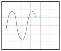
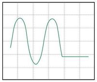
Various scope trace possibilities with (a) bias too high, (b) bias too low, and (c) bias set to optimal sensitivity for out-of-contact.
| ||
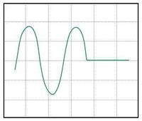
The software plots amplified detector output voltage on the y-axis, and stage actuation signal voltage on the x-axis. Watching these signals in the software and on the oscilloscope in x-y mode you should see something like the plots shown in Figure 8: a flat line that breaks into a $ sin^2 $ function at a certain x-value. The flat line is the cantilever out of contact, and the oscillating section is the cantilever bending, after making contact with the sample. You will see that as the piezo moves the sample down it pulls the tip through the original point of contact, and the oscillations of the diffractive transducer continue on-screen. This is because there is always an adhesion force between the sample and the probe tip. The stage must move a certain distance away, thereby applying a certain force, to break contact. If the humidity is high, or the sample and tip simply have a high affinity toward one another, this adhesion can be quite sever. Depending on your resolution, you may also see these attractive forces as a small bump in photodiode signal just before the sample makes contact with the probe tip as the stage travels back up.
To determine the sensitivity of stage movement to x-axis voltage, voltage applied across the piezo disc, we can take advantage of the fact that a mode's brightness goes from fully bright to fully dim (peak to trough on the $ sin^2 $) as the fingers deflect through an actual distance of $ \lambda/4\approx 160 nm\,\! $. With this in hand, you can now calculate the relationship between relative finger deflection and y-axis voltage, photodiode voltage, in nm/V. Don't forget the gain in the AM502.
In addition you will also need to multiply the sensitivity by a correction factor $ A_{corr} $ to account for the location of the diffraction fingers with respect to the tip of the cantilever. $ A_{corr} $ can be estimated most simply by assuming a quadratic shape for the bent cantilever $ A_{corr} $ = 1/m$ ^2_{ID} $, where m$ _{ID} $ = L$ _{ID} $/L$ _{T} $ is the ratio of the distance of the ID fingers from the cantilever base to the total cantilever length. However, a more precise expression for imaging, derived from the equation for the shape of a simple rectangular beam with an applied end-load, is $ A_{corr} $ = 2/(3m$ ^2_{ID} $ - m$ ^3_{ID} $). And for out-of-contact measurements such as the thermal vibration experiment it is more appropriate to think of the beam as being loaded by its own weight, a distributed load, so in that case a more precise expression is $ A_{corr} $ = 3/(6m$ ^2_{ID} $ - 4m$ ^3_{ID} $ + m$ ^4_{ID} $).
Biasing
It is critical to properly bias the diffraction transducer and helpful to properly choose a set-point if you will be imaging. First, use the offset on the voltage amplifier to position the sin$ ^2 $ so that it is centered around zero. Next set the out-of-contact bias by moving the position of the laser spot on the fingers until the flat section of the photodiode output curve is approximately at zero volts, halfway between the maximum and minimum, as in Figure 8c. This is also the point of maximum sensitivity for the diffraction transducer. This process is possible because the fingers are slightly bent, as described in Optical system, and we are simply finding a desired spot of relative-finger-displacement when the cantilever is in a state of zero-deflection.
Finally, for best results imaging a sample, a set-point must also be chosen. Set-point is defined as the distance you will move the stage past the contact point when engaging on a sample. This will apply a small force so that contact is maintained even when scanning over valleys in your sample, and will also match the transducer's point of calculated sensitivity with the average sample topography height. The set-point can be initially chosen equal to the estimated average amplitude of features on the sample and revisited for later samples. It is set in this calibration procedure by moving the laser spot so that the point of maximum sensitivity is arrived at a small distance after the point of contact on the photodiode output curve. Thus the correct imaging bias will look like Figure 8b; i.e., you will be moving the the flat portion of the detector output down on screen.
Software
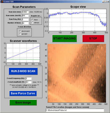
The software that interfaces with the AFM is an application that runs in matlab. It is found in the course locker under "Labs\AFM\trunk" and its graphcial user interface (GUI) is launched by typing 'AFMControlPanel' in the matlab command window (caps needed). Its main function is to systematically scan the probe tip back-and-forth across the sample, recording the cantilever deflection information at each point, line by line, and assemble that data into an image. Figure 9 shows a screen capture of the scanner control window. However, it also allows the user to do a z-mod scan. An overview of its operation is provided below.
Controls overview
Many of the are self-explanatory, such as the start imaging and stop buttons, as well as the image area in the lower right, which displays the image currently being scanned. Some notes are given below on features that are not immediately obvious.
To begin with, it's easiest to simply use the default settings on all these controls, and to experiment with changing them as you become more familiar with the tool.
Scan Parameters - The Scan size sets the length and width of the image in nanometers (always a square shape), but its accuracy depends on having the correct value for "Scan sensitivity" (from your calibration procedure). The "Scan frequency" (lines per second) sets the speed of the tip across the surface, and together with the number of lines affects the amount of detail you will see in the image. Setting the Y-scan direction tells the scanner whether to start at the top or the bottom of an image, and the trace/retrace selector determines whether each line is recorded as the tip scans either to the left or to the right.
Scope View - As the tip scans back and forth, this plots the tip deflection data for each line. It is useful for quantitative feature height measurements.
Scanner Waveforms - Shows the voltage waveforms driving the piezo scanner, for each scan line that is taken. This is helpful for knowing where in the image the current scan line is located, and for knowing the output level of the waveforms driving the scanner.
Z-mod Controls - These are only active during a z-mod scan, and have no effect when taking an image. For more on this mode, see Z-mod (force spectroscopy) operation.
Image mode operation
This is the primary operating regime of the AFM, and provides a continuous display of the surface being scanned, as the probe is rastered up and down the image area. To use this mode, the switch on the back of the AFM must be flipped upward. Remember that the maximum scan area is only abut 15 $ \mu $m square, and adjusting the position of the sample under the tip requires only the smallest movements of the stage micrometers. Finally, keep in mind that there is always a delay after pressing start imaging before the scan begins, as the actuator drive signals are buffered to the I/O hardware.
Z-mod (force spectroscopy) operation
In this mode, the piezo moves the sample only along the z-axis; i.e., straight up and down (hence z-mod, short for z-modulation). To use this mode, the switch on the back of the AFM must be flipped downward. The defaults for frequency and amplitude, 2 Hz and 8 V, provide a nice force curve. Besides being critical for calibrating and biasing the readout, this mode is used to perform force spectroscopy experiments, in which tip-sample forces can be measured as the tip comes into and out of contact with the sample.
(Note that the red stop button is also used to stop a z-mod scan).
Saving AFM data
The software allows you to save the raw data of both images as well as force curves. Not surprisingly, the "Save Image" and "Save Force Curve" buttons do this. In both cases an instantaneous snapshot of the current image or force curve is written to the file location specified in the entry box at the bottom of the window.
An image is written to a files as a square matrix (interpolated to have the same number of rows and columns), with the value at each point representing height data. Force curve data is saved as two columns: x-axis (stage deflection) data in column one, y-axis (mode intensity) in column two.
If you intend to save an image, it is best to set the filename before starting the scan — the filename box behaves $ \ldots $ elusively while the scanner is running due to some peculiarities of the software.
As a final note, a "quick and dirty" way to save an image is by simply doing a screen capture while the AFM is scanning (press \Print Screen" on the keyboard). The captured image can then be pasted into MS Paint (Programs $ \rightarrow $ Accessories $ \rightarrow $ Paint) and cropped to leave only the scanned AFM image. These images can be imported into matlab for analysis/processing (we'll do this in later parts of the course).
Additional instrumentation
Differential amplifier
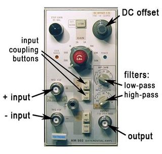
The Tektronix AM502 is a differential amp, so it amplifies the voltage difference between the two input signals. Both inputs have DC, AC, and GND input coupling, like the scopes. The amp can be used single-ended if the (−) input is left unconnected and ground-coupled. The gain (amplification factor) ranges from 1 to 10,000, and is set by the red knob together with the "÷100" button above it. The instrument also has high- and low-pass filters. These are somewhat confusingly labeled "HF-3dB" and "LF-3dB" (see Figure 10). This doesn't mean \high-pass" and \low-pass," but refers to the "high [cutoff] frequency" of a LPF and the "low [cutoff] frequency" of a HPF. Therefore, HF-3dB is the low-pass filter, and LF-3dB is the high-pass filter.
Both filters are considered "off" when the low-pass is turned all the way up, and the high-pass all the way down.
Finally, the lower (high-pass) filter knob also has two settings for controlling output signal DC level: dc and dc offset. When set to dc, the amp outputs the actual DC level of the input signal, multiplied by the gain. Set to dc offset, you can manually adjust the DC level using the knob at the upper right of the AM502. In both cases, the AC component is simply added on top.
LabVIEW VIs for signal capture
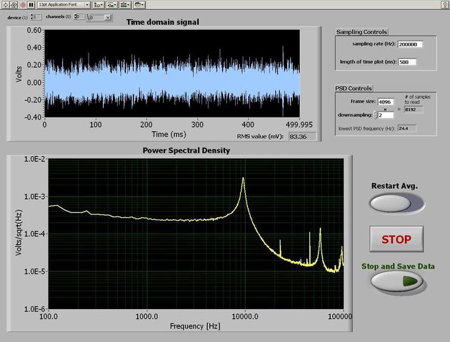
The spectrum analyzer
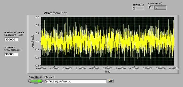
Time-domain signal capture
Experiment 1: Mini-lab: Measuring cantilever stiffness
Theory: thermomechanical noise in microcantilevers
For simplicity of analysis, we model the cantilever as a harmonic oscillator with one degree of freedom, similar to a mass on a spring, as discussed in lecture. According to the Equipartition Theorem, the thermal energy present in the system is simply related to the cantilever fluctuations as follows: foo
where $ z^2 $ is the mean-square deflection of the cantilever, $ T $ is the absolute temperature, $ k $ is the cantilever spring constant, and $ k_B $ is Boltzmann's Constant (yes, this notation can be confusing so take care to keep these $ k $s straight).
The square root of the PSD for this second-order resonant system is
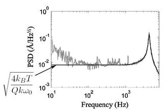
in which $ \omega_o $ and $ Q $ are the (angular) resonant frequency and quality factor, respectively. In order to understand how this function is derived, it is recomended that you see M. Shusteff, T. P. Burg, and S. R. Manalis, "Measuring Boltzmann's constant with a low-cost atomic force microscope: An undergraduate experiment," Am. J. Phys. 74(10), pp. 873-9, (2006). In the paper the authors calculate the cantilever stiffness and use it to estimate Boltzmann's Constant, as an interesting exercise. We will actually do the reverse: measure the cantilever stiffness using Boltzmann's constant. This procedure is used quite extensively because in practice it is exceedingly difficult to accurately measure the geometry and precise material properties of the cantilever. Note that at low frequencies ($ \omega \ll \omega_o $), this expression yields called the "thermomechanical noise limit" for displacement detection (see Figure 13 for an illustration):
These relations suggest several possible approaches that can be taken for determining $ k $, for which you will need to know (1) the quality factor Q and resonant frequency $ \omega_o $ of the resonator, and (2) either the low-frequency limit of the PSD or the mean-squared deflection.
- The quality factor and resonant frequency can be obtained from measuring the noise PSD of the vibrating cantilever. If your intuitive sense for them is good, you can estimate these quantities directly from the plot, or determine them more precisely by fitting an ideal PSD to the noise data (more on this in Data analysis in MATLAB).
-
The mean-square deflection is readily available from either time-domain or PSD data of the cantilever thermal noise. Recall that these are related through Parseval's theorem as follows:
$ \big\langle\Delta z^2 \big\rangle = \textstyle \int\limits_{0}^{\infty} S(\omega)\, d\omega $,
where S(ω) is the PSD function of \Delta z. By now, you know enough MATLAB spectral analysis techniques to make these calculations. You will likely find that simply using the mean-square noise value and Parseval's theorem will not give you a good result (why?). Instead, the approach in Data analysis in MATLAB will work much better.
Other methods of estimating cantilever stiffness
The spring constant (stiffness) can be analytically calculated from geometrical parameters in two ways (see Cantilevers for thermal noise measurements and Figure 5 and Figure 6 for cantilever dimensions). From basic mechanical beam-bending analysis of a rectangular cantilever the stiffness k can be expressed as
in which E is the elastic (Young's) modulus of the beam material, and L, b and h are the length, width, and thickness of the beam, respectively (b is used for the width to avoid confusion with angular frequency !ω). This method, however, does not always yield accurate results — can you suggest why?
Another analytical model for the spring constant was devised by Sader and coworkers[1], and it relies on measuring the cantilever's resonant frequency:
where ρ_c is the mass density of the material, L, b, and h are the same geometrical parameters as above, and $ \omega_{vac} $ is the cantilever's resonant frequency in vacuum. For the purposes of these calculations, you can assume that the resonant frequency you will measure in air, $ \omega_{air} $, is 2% lower than $ \omega_{vac} $. (remember the factor of 2π when converting between ω and f in your equations).
Suitable material parameters to use for the low-stress silicon nitride ($ Si_xN_y $), out of which these cantilevers are made are ρ_c = 3400 kg/$ m^3 $, and E = 250 GPa. Dimensions are given in Cantilevers for thermal noise measurements
Thermal noise calibration and biasing using the cantilever pairs
For the accuracy of this measurement, it's especially important that the signal be biased at the maximum-slope position along the output curve when it's not in contact with the surface.
By now you're familiar with aligning, calibrating, and biasing your AFM. The major difference in this case is how you'll actually perform the z-modulation scan for the calibration.
Because this device is a pair of identical cantilevers, simply bringing it down to a surface will deflect both beams equally. A z-mod scan will show approximately zero deflection of one beam relative to the other. Instead, we want to bend only one of the beams, while keeping the other unbent.
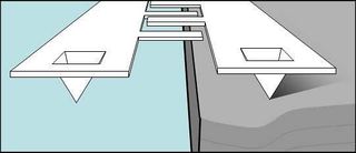
To do this, you'll use a sample with a sharp step edge. The goal is to position the cantilever pair above this edge such that one of the beams will be on the surface, and the other will hang in free space (sketched in Figure 14). A z-mod scan should then deflect only one of the beams, giving us the calibration curve we want. (Note: reflections of the laser from the edge of the substrate can interfere with the diffractive modes. If this is the case, try repositioning the sample edge, perhaps using only the corner to bend one of the cantilevers, until the $ sin^2 $ shape improves.)
Recording thermomechanical noise spectra
Once you're satisfied with your calibration and bias point, withdraw the lever's tip from the surface, making sure that the bias point stays where you set it. Gain up the signal using the AM502 voltage amp, and use the LabVIEW spectrum analyzer to record the thermal noise signal coming from the freely vibrating cantilever. Once you are happy with how the spectrum looks, save it to a .txt file of your choice.
You only need to measure the noise spectrum down to about 50-100 Hz. Below this frequency, 1/f-type or "pink" noise dominates. You are welcome to measure this if you are interested, but it is of limited use for determining $ k_B $. For very low-frequency measurements, anti-aliasing and proper input coupling becomes very important. If you are interested in this, your lab instructor can provide guidance.
Some guidelines for getting a good noise spectrum:
- Choose a sampling frequency at least 2× higher than the highest frequency of interest, or about 10× higher than the first resonance peak of the cantilever.
- Use AC coupling on your voltage amplifier, and use a gain of 100-1000.
- If necessary, add a low-pass anti-aliasing filter (recall from the DNA Melting Laboratory) at an appropriate frequency to eliminate high-frequency components being "folded" over into the frequency region of interest.
- Recall from the previous lab that, if you prefer, you can also measure the time-domain signal directly, and later calculate its PSD in MATLAB. You can decide which technique you prefer.
Data analysis in MATLAB
Once you bring your saved PSD data from LabVIEW into matlab ([Fvec,PSDvec]=load(`filename') is the syntax you want), you can manipulate it as you wish. To fit the second-order transfer function $ G(\omega) $ to the noise data, we'll use the lsqcurvefit routine from matlab's optimization toolbox. We're aiming to do something similar to what you see in Figure 13, where an ideal function is overlaid on real noise data.
To make the fit converge easily, we'll separate the nonlinear f_o and Q parameters from the linear scaling factor. When doing the fitting, it is helpful not to use the whole frequency range of your data. Instead, crop your PSD data to a suitable range around the resonant peak — the vectors xdata and ydata used below are cropped PSD frequency and magnitude data, respectively, extracted from Fvec and PSDvec.
First, you'll need the matlab function transfunc to generate the unscaled transfer function (i.e. the thermomechanical noise scaling factor is 1 here — refer to the equations in Theory: thermomechanical noise in microcantilevers):
The function takes the f_o (note that this is real frequency in Hz, and not angular frequency in rad/sec) and Q parameters as input, with a vector of frequencies, and outputs corresponding PSD magnitude data:
    function [output]= transfunc(params,xdata)
    % params [f_o Q]
    x=xdata/params(1); % x-matrix to contain freq. points normalized to f/f_o
    output=sqrt(1./((1-x.^2).^2 + (x/params(2)).^2));
Then, create a function scaling to do the linear scaling, and calculate the thermomechanical noise level (the left-divide operation actually does a least-squares fit):
    function [y]=scaling(params,xdata,ydata)
    unscaled=transfunc(params,xdata);
    A=unscaled\ydata; % note the left-divide here!
    y=unscaled*A;
Finally, use the lsqcurvefit routine, supplying an appropriate initial guess for f_o and Q:
    options=optimset(`TolFun',1e-50,`tolX',1e-30);
    p=lsqcurvefit(`scaling',[f_guess Q_guess], xdata, ydata, [ ], [ ], options, ydata);
This will return the best f_o (again in Hz, not in rad/sec) and Q parameters after the fit as a two-element vector p. Now you just need the scaling pre-factor, which you can get by left-dividing the full-range fit function by the PSD magnitude data (the left-divide again gives you a least-squares fit "for free"):
A=(transfunc(p,full_xdata))\full_ydata;
Here full_xdata and full_ydata are the full-range frequency and magnitude PSD vectors, rather than just the cropped sections used for the fit algorithm. You can now see how well the fit worked, by plotting it on top of the original PSD data:
Gfit = A*transfunc(p,full_xdata); loglog (full_xdata, Gfit);
Experiment 2: Imaging
The general approach to imaging is to (1) set the overall output signal range and offset while in the z-mod regime, (2) stop the z-mod scan and engage the probe with the surface, and (3) carefully adjust the cantilever deflection to give the desired bias point, and (4) start the image scan.
Correct biasing is key to obtaining good images. If you are not yet comfortable with choosing and setting an appropriate bias point for the cantilever's optical readout, it is worth reviewing that material from Calibration and biasing.
For imaging, maximum out of contact sensitivity is not the goal. Instead, the sensitivity should be greatest when the probe is engaged, and exerting a small force on the surface. The more force the probe applies to the surface, the more wear and damage to the probe and surface can result.
The samples available for imaging are calibration gratings, various integrated circuit chips, and E. coli bacteria on a silicon dioxide surface. With the latter two, you may need to navigate around the surface in order to find interesting features to image. Unfortunately, unlike commercial instruments, our AFMs do not have an integrated optical viewing system, so when positioning the sample it is difficult to determine exactly what spot on the sample the probe tip will scan. Use the stereo-microscope (at moderate magnification) and a fiber-light to observe the tip and position it as well as you can. Temporarily turning off the sensing laser will make it easier to see. You can move the sample "on the fly", as you're imaging, but it takes some practice to make small enough stage movements. You will also likely have to readjust the bias point (also fine to do on the fly).
AFM resolution limit
Researchers using the AFM always need to know their noise-limited resolution. Therefore, we will characterize the noise floor of the system, so we know what performance to expect.
The simplest way to do this is to look at the root-mean-square (RMS) noise, which represents the average fluctuations that will obscure features in AFM images. RMS noise data is easily obtained by recording a length of the output signal in the time domain (using the VI from LabVIEW VIs for signal capture), and analyzing the data in matlab.
You should capture and calculate the RMS noise of the AFM both out of contact and in contact with the sample surface. Make sure you don't lose your calibration, especially when you bring the AFM into contact — it's easy to move to a different point on the output curve.
You may also find it instructive to look at the noise output signal using a Spectrum Analyzer (LabVIEW VI in LabVIEW VIs for signal capture) to see whether the noise is concentrated in particular spectral regions.
Experiment 3: Elastic modulus
[For these measurements, we'll use the shortest and stiffest cantilevers available to us, which will give the best signal. These have very similar geometry to the long cantilevers in Figure 5, but have a length of 250 μm, and a width of 50 μm. The fingers begin 43 μm from the base and end 125 μm from it. Ask your lab instructor to provide you with a short cantilever when you are ready.]
As you may know, some of the most useful applications of AFMs in biology take advantage of their ability to measure very small forces. We'll use this capability to measure the elastic moduli of some soft samples, to simulate mapping cell wall elastic properties, similarly to the 2003 paper by Touhami et al.[2]
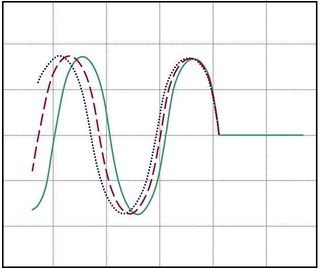
As seen in this paper, when using the optical lever sensor, samples with different elastic moduli change the slope of the in-contact portion of the force curve. For our non-linear ID sensor, the equivalent of changing the slope is a changing period for the $ sin^2 $ function. Just as softer samples cause lower slope with the optical lever, softer samples give the output function of the ID sensor a longer period, with greater spacing between the peaks (see Figure 15(a) below).
The approach for measuring modulus is to first take a force curve on a reference sample, considered to have infinite hardness. We will use a bare silicon nitride surface. This allows us to determine how the x-axis signal corresponds to stage movements.
You'll want to bias this measurement similarly to measuring noise — the output should be at the middle of the output range when out of contact (See Figure 15(b)).
After your measurement of the hard sample, switch to the more compliant PDMS elastomer samples, and run force curves on them.
Make sure to save these force curves for later analysis, described in Elastic modulus data analysis.
To get good force curves:
- Don't change the biasing or laser position between samples — if you do, the force curves you get can't be compared one to another.
- Careful initial biasing at the middle of output range is worth it — this will make a big difference in ease of data analysis.
- After you've brought each sample into contact and are satisfied with the Z-modulation range, run the scan at slow speed (e.g. 0.5Hz) for the cleanest force curves.
Elastic modulus data analysis
According to Touhami et al., the depth δ of an indentation made by a conical tip (approximately true for ours) is related to the applied force $ F $ by
where α is the half-angle of the mostly-conical end of the pyramidal tip, and $ E $ and ν are Young's elastic modulus and the Poisson's ratio of the substrate material, respectively.
Substituting in appropriate values for α (35.3°) and ν (0.25), we are left with
in which we need only the force and indentation δ values to calculate modulus.
The force $ F $ is calculated by treating the cantilever as a Hookian spring, which obeys the law $ F = -kz $, where $ k $ is the spring constant and $ z $ the tip deflection. For the 250 μm long cantilever, assume a spring constant of 0.118 N/m.
Finally, all that remains is to calculate indentation depths for the soft materials from the difference in the period of the $ sin^2 $ output between their force curves and the one for the hard sample. Corresponding forces are derived from the cantilever deflection. Don't forget at all points to include the factor that relates cantilever tip deflection to finger deflection.
Experiment 4: Protein pulling
If you wish to do an experiment in protein pulling, talk to your instructor.
Report requirements
DISREGARD THESE for the Limits of Detection mini-lab.
Calibration and noise
- For each measurement you perform, briefly describe the calibration you carried out, and the calculations for the calibration factor in each case. Remember to take into account any amplifier gain, geometric factors, etc. that affect the value of the signal.
- Using your calibration factor, determine the RMS noise of the system both in and out of contact, in nanometers. Are there particular spectral regions at which noise is greatest?
- Based on your calculations, can these AFMs resolve atoms? What about DNA? Large globular proteins? Cells?
Measuring Boltzmann's constant
- Carry out the data analysis of Data analysis in MATLAB and summarize your results with a plot showing the noise spectra for the cantilever you chose and the fit functions for them. Include the relevant matlab code.
- Your report should include the values of spring constants $ k $, resonant frequencies $ f_o = \omega/2\pi $, and quality factors $ Q $, that you found for both cantilevers.
- Explain which method of calculating spring constant you preferred, and why.
- Are these methods actually accurate? If not, can you suggest a better approach?
- What value of Boltzmann's Constant $ k_B $ did you find. Note, you may use more than one device type and/or size. If you do, report all results here.
- How close were you able to come to the actual value of $ k_B $, which is 1.38×10$ ^{\mbox{-23}} $J/K? (You will be graded much less on the accuracy of your $ k_B $ value than on the quality of your analysis.)
- Error sources are the most important consideration in any instrumentation and measurement endeavor. Consider the sources of uncertainty and "noise" in this experiment, and in so doing demonstrate an understanding of the factors that influence the accuracy of your measurement:
- Calibration accuracy
- Geometrical correction factor
- Spring constant calculations, including geometrical ($ L, b, h $) and material ($ \rho_c, E $) parameters
- Parameters derived from the PSD curve fit ($ Q $, $ \omega_o $)
- Any noise in the system other than thermally-driven vibrations of the cantilever beams
- You should estimate the uncertainty/noise in these various components and steps of the $ k_B $ calculation (if you aren't sure how to approach this, you'll probably find it helpful to discuss with your lab instructor). Paragraphs of explanation for all item are not necessary - focus on the major sources of error/uncertainty.
- Questions that will help you:
- How confident can you be of the various values that we take as given? Within ±10% or ± a factor of 2. If a particular variable has a 20% error, how does that propagate to $ k_B $; i.e., what's the dependence of $ k_B $ on that variable?
- Based on these estimates, which one or two items dominate the error in the measurement? (i.e. improving anything else won't help until this dominant source of error/uncertainty is dealt with).
Imaging
If you do the imaging experiment, report these additional items:
- Choose 2-3 samples from those available. For each one, center on an area or feature of interest (e.g. a single E. coli bacterium) and take a high-resolution scan (at least 1 Hz and 32 lines - but go as fine as you like). This scan should be approximately 3-5 μm square. Include a capture of this scan in your report (Preferably your image is captured as a file and processes MATLAB techniques you learned in this class. Be careful not to remove important information).
- Determine the lateral (x- and y-axis) dimensions and the vertical (z-axis) height of the object or feature. Indicate these either directly on the image, or in the image caption/description.
- Comment on what you think the resolution limit of your AFM is (lateral and vertical). Your noise measurements should help your thinking. How small of a "bump" can be resolved? How does the slope of the bump edges affect this?
- (BONUS) Time permitting, try scanning very fast (10Hz or more — WARNING, this may cause some unpredictable results). How does this affect resolution, image quality and stability, and other performance considerations?
Elastic modulus
If you do this experiment:
- Calculate and report the elastic modulus of two different elastomer samples and to determine which is softer.
- Analyze and write about sources of error that are unique to this measurement, in addition to the error sources discussed in the rest of your report.
Protein pulling
Talk to your instructor about reporting requirements for this experiment.
Lab problems
Force resolution
In lecture, we discussed the minimal force detectable with a microcantilever. The force was assumed to have a white spectrum, and its PSD (at all frequencies) had a value of:
Using analytical expressions for spring constant and resonant frequency, given by
answer the following questions:
- (a) Calculate the minimum detectable force in a 100 Hz bandwidth using the 350 μm beams from this lab.
- (b) How does this value compare to typical forces in biological systems (e.g. antibody/antigen binding, DNA hybridization, interdomain forces in proteins, etc.)? Use whatever knowledge you may have, or find one or two examples, but don't spend too long doing literature searches.
- (c) Which cantilever geometrical parameters affect the minimal detectable force? I.e. for smaller forces, do you need a cantilever that's shorter? thinner? wider? Comment on which parameter variations will have the greatest effect.
Useful resources
AFM basic operating principles
- A website with a basic description:
- One with some more detail:
- If these really stimulate your interest, this is a more comprehensive site on Scanning Probe Microscopy (SPM), of which AFM is a subset:
- The paper that started it all: G. Binnig, C. F. Quate, Ch. Gerber, "Atomic Force Microscope" Physical Review Letters 56(3):930-933, 1986.
Using interferometric ID fingers for position detection
- The original paper:
- A more thorough treatment:
A nice review of using the AFM in biology
References
- ↑ J. E. Sader, et al, "Calibration of rectangular atomic force microscope cantilevers," Review of Scientific Instruments, 70(10):3967-3969, 1999
- ↑ A. Touhami, B. Nysten, and Y. F. Dufrene, "Nanoscale Mapping of the Elasticity of Microbial Cells by Atomic Force Microscopy," Langmuir 19(11), 4539-43 (2003).

