Difference between revisions of "Assignment 8, Part 0: convolution practice"
From Course Wiki
Juliesutton (Talk | contribs) |
|||
| (9 intermediate revisions by 3 users not shown) | |||
| Line 1: | Line 1: | ||
| + | <noinclude> | ||
| + | |||
[[Category:20.309]] | [[Category:20.309]] | ||
[[Category:Lab Manuals]] | [[Category:Lab Manuals]] | ||
[[Category:DNA Melting Lab]] | [[Category:DNA Melting Lab]] | ||
{{Template:20.309}} | {{Template:20.309}} | ||
| + | |||
| + | </noinclude> | ||
| + | |||
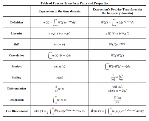
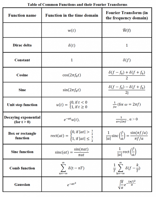
| + | The following two tables will pop up frequently in 20.309 for the rest of the semester. Table 8.0.1 describes the Fourier transform and many of its useful properties, while table 8.0.2 contains the transform pairs of many common functions. These two tables are useful because you can combine functions in table 8.0.2 using the properties in table 8.0.1 to figure out the transforms of an endless number of functions (without doing any math!). | ||
| + | |||
| + | Note: there is an error in the table below. The transform of <math>u(t)</math> is: <math>\frac{1}{2}\left ( \frac{1}{i \pi f}+\delta (f) \right )</math>. | ||
| + | |||
| + | [[Image: FourierTransformsTable.png|thumb|left|500 px|<caption>Table 8.0.1: Short table of Fourier transform properties</caption>]] | ||
| + | |||
| + | [[Image: TimeFrequencyDomains_MoreTransformPairsTable.png|thumb|left|500 px|<caption>Table 8.0.2: Short table of Fourier transform pairs</caption>]] | ||
| − | {{Template:Assignment Turn In|message= | + | {{Template:Assignment Turn In|message= |
| − | + | ||
| − | + | ||
| − | + | ||
| − | + | ||
| − | + | ||
| − | + | ||
| − | + | ||
| − | + | ||
| − | + | ||
| − | + | ||
| − | + | ||
| − | + | ||
| − | + | ||
| − | + | ||
| − | + | ||
| − | + | ||
| − | + | ||
| − | + | ||
| − | + | ||
<ol type="A"> | <ol type="A"> | ||
| + | |||
| + | <li>Sketch each function in table 8.0.2 as well as the magnitude of its Fourier transform. Include any relevant constants in your sketch (for example: ''a'', <math>\alpha</math>, and <math>f_0</math>). | ||
| + | </li> | ||
| + | <br> | ||
<li> | <li> | ||
| − | In class we found the Fourier transform of <math>\cos^2(\omega_0 t)</math>. Use graphical convolution to determine the transform of <math>\cos^4(\omega_0 t)</math> | + | In class we found the Fourier transform of <math>\cos^2(\omega_0 t)</math>. Use graphical convolution to determine the transform of <math>\cos^4(\omega_0 t)</math>. |
</li> | </li> | ||
<br> | <br> | ||
| Line 36: | Line 33: | ||
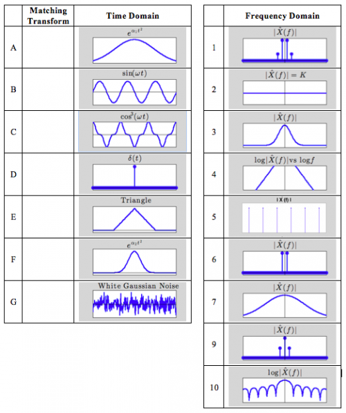
<li> Table 8.0.3 shows plots of eight time-domain signals A-H. The table on the right includes magnitude plots of the Fourier transform of ten signals numbered 1-10. For each time domain signal A-H, write the number 1-10 in the empty column of the matching frequency-domain signal. You may use a numbered plot more than once.<br> | <li> Table 8.0.3 shows plots of eight time-domain signals A-H. The table on the right includes magnitude plots of the Fourier transform of ten signals numbered 1-10. For each time domain signal A-H, write the number 1-10 in the empty column of the matching frequency-domain signal. You may use a numbered plot more than once.<br> | ||
Some of the frequency plots are shown on log-log axes and some are linear, as indicated by the plot title.<br> | Some of the frequency plots are shown on log-log axes and some are linear, as indicated by the plot title.<br> | ||
| + | ''Hint:'' Gaussian or white noise is a random signal with equal contributions from ''every frequency''. | ||
| − | |||
</li> | </li> | ||
<br> | <br> | ||
| − | </ol> | + | </ol>}} |
| − | + | ||
| + | [[Image: PSet4_ConvolutionImage.png|thumb|center|500 px|<caption>Table 8.0.3</caption>]] | ||
| + | |||
| + | <noinclude> | ||
{{Template:Assignment 8 flow channel & two-color microscope navigation}} | {{Template:Assignment 8 flow channel & two-color microscope navigation}} | ||
{{Template:20.309 bottom}} | {{Template:20.309 bottom}} | ||
| + | </noinclude> | ||
Latest revision as of 17:44, 13 October 2022
The following two tables will pop up frequently in 20.309 for the rest of the semester. Table 8.0.1 describes the Fourier transform and many of its useful properties, while table 8.0.2 contains the transform pairs of many common functions. These two tables are useful because you can combine functions in table 8.0.2 using the properties in table 8.0.1 to figure out the transforms of an endless number of functions (without doing any math!).
Note: there is an error in the table below. The transform of $ u(t) $ is: $ \frac{1}{2}\left ( \frac{1}{i \pi f}+\delta (f) \right ) $.
- Overview
- Part 1: feedback systems
- Part 2: fabricate a microfluidic device
- Part 3: add flow control and test your device
Back to 20.309 Main Page


