20.109(S23):M2D6

Introduction

Diagram of a fluorescence microscope.

In the previous lab session, antibody staining was used to identify expression of Fet4_mutants in yeast. The first antibody, or primary antibody, was anti-V5 tag and raised in a mouse. This antibody is conjugated to a fluorescent dye tag called Alexa Fluor 488, eliminating the need for a secondary antibody to visualize the staining. The Alexa Fluor 488 tag is a green fluorescent dye that is excited at 488 nm. To visualize the expression of your tagged mutant Fet4, we will use fluorescence microscopy.

In fluorescence microscopy the specimen is illuminated with a wavelength of light specific to the excitation of the fluorescent tag used to target the feature of interest. The excitation wavelength is absorbed by the fluorescent tag, which causes it to emit light at a longer, less energetic wavelength. Typically, fluorescence microscopes used in biology are an epifluorescence type with a single light path (the objective) for excitation and emission detection, as depicted in the diagram above.

Fluorescence, or epifluorescence, microscopes are composed of a light source, an excitation filter, a dichroic mirror, and an emission filter. The filters and the dichroic mirror are specific to the spectral excitation and emission characteristics of the fluorescent tag. To visualize fluorescence, light at the excitation wavelength is focused on the sample. The light emission from the sample is focused by the objective to a detector.

In this lab session, you will also perform the metal uptake experiment, as discussed in prelab. This data will be analyzed and discussed in more detail in the following lab session.

Protocols

Part 1: Induce expression of Fet4_mutant

For timing reasons, the induction steps were completed prior to class. So you understand how the cell suspensions you will use for the metal uptake assay were created, please review the steps below.

1. Inoculated 5 mL of SD-R media with a colony of Alpha = W303α cells transformed with Fet4_mutant.
2. Incubated the culture overnight at 30 °C with shaking at 220 rpm.
3. Dilute the overnight culture 1:10 in 10 mL of fresh SD-R media.
4. Incubate at 30 °C for 4 hours with shaking at 220 rpm.
5. To induce Fet4_mutant protein expression, pellet cells and resuspend in 10ml of SD-G media.
6. Incubate overnight at at 30 °C with shaking at 220 rpm.

Part 2: Perform metal uptake experiment

1. Obtain W303α transformed with Fet4_mutant culture from the front bench
2. While you prepare the experiment with your mutant, the instructors will prepare controls using the following cultures:
   • Untransformed W303α
   • W303α transformed with Fet4
3. Gently tritruate with a 1ml pipette to create a homogeneous suspension for each culture
4. Obtain cuvettes from the front bench to measure the OD₆₀₀ of each culture prior to beginning the experiment
5. Add 1ml of each cell suspension to individual cuvettes and read on the spectrophotometer
   • Use 1ml SD-G for a blank.
6. Record these numbers in your notebook
7. Using SD-G media as a diluent, dilute each of your cultures to OD₆₀₀ ~ 1.0 and a final volume of 8ml. This does not have to be exact, but the cultures should have a similar OD₆₀₀ before you begin the experiment.
8. Add CdCl₂ and FeCl₂ for final concentration of 100μM in each culture and add to a new glass tube.
9. Incubate your labeled glass tubes shaking at 30°C for 2.5 hours to allow uptake.
   • During this incubation time, complete Parts 3 of the wiki.
10. Following incubation, take an additional OD₆₀₀ reading to account for any changes in culture density, and allow normalization of data across groups.
    • Record this in your notebook.
11. Transfer your cultures to 15ml conical tubes.
12. Centrifuge cultures at 1000 xg for 5 minutes to pellet cells.
13. During centrifugation, label 2 metal-free 15ml conical tubes for your mutant culture, and prepare a 10ml syringe filter for each culture
14. Using serological pipette, remove 6ml media supernatent without disrupting the pellet and add it to a metal-free conical tube.
15. Bring your samples to the front bench and add 175ul ultra-pure nitric acid to each sample. Return to your bench with your samples.
16. Using a serological pipette, carefully triturate each sample to fully mix the acid.
17. Open your 10ml filter syringe and place it over the top of a fresh metal-free conical tube. Add the mixed sample to the open syringe and use the plunger to push the sample through the 0.22 μM filter.
18. Close each tube with sample and place them at the front bench.
19. Discard materials used to filter the samples in the black bin at the front bench.

In your laboratory notebook, complete the following:

• What volume of CdCl₂ will you add to obtain a final concentration of 100 μM?
• What volume of FeCl₂ will you add to obtain a final concentration of 100 μM?
• Why is it important to use metal-free tubes to store your samples for analysis?
• Why is it important to filter your samples before submitting them for analysis?

Part 3: Examine example Fet4 mutant expression

Qualitatively assess signal localization and quantify total FITC intensity for all images Please obtain the raw Fet4_mutant expression images from the dropbox folder on the class data page. Three sets of images (i.e. image stacks) were taken per experimental condition, and each image stack contains images from two channels: DAPI (blue) and FITC (green). Remember that the V5 primary antibody used for the Fet4_mutant staining was conjugated to an Alexa4888 fluorophore, which emits green light. For each image stack, you will use ImageJ to 1) identify the location of the nuclei using the DAPI channel and 2) broadly assess the Fet4_mutant fluorescence in the FITC channel at locations specified by the DAPI channel. These images were taken at 40x magnification.

First, you will identify the total FITC signal intensity for each image.

1. Open ImageJ.
2. Open one image stack from the Fet4 condition.
   • The first image you see is the DAPI channel
   • If you scroll to the right, the second image in the stack is the FITC (V5-tagged Fet4) channel.
3. Using the DAPI channel to orient yourself, examine the FITC signal localization for the image and use the questions below to note your qualitative assessment of the signal localization.
4. Repeat this assessment for the remaining experimental groups

In your laboratory notebook, complete the following:

• What is your qualitative assessment of the yeast cells and Fet4 localization for each condition?
  • Are all nuclei approximately the same size and shape?
  • Can you identify FITC signal in the cell (i.e. is the FITC channel have signal roughly around DAPI channel)?
  • Do you see FITC signal where you expect?
  • How might you generate images that can provide more qualitative information?

Part 4: Quantify Fet4 mutant expression

Quantify total FITC intensity for all images While qualitative data is valuable to determine protein localization, quantitative data can also provide useful information about expression levels of your protein of interest. Here you will determine a quantification of signal intensity which can be used as an approximation of protein expression in the culture.

To do this, you will identify the total FITC signal intensity for each image.

1. Open ImageJ.
   • Go to Analyze -> Set Measurements.
     • In the Set Measurements window, make sure the following boxes are checked: Area, Mean gray value, Min & max gray value, Shape descriptors, Integrated density, Display label.
2. Open one image stack from the no treatment condition.
   • The first image you see is the DAPI channel
   • If you scroll to the right, the second image in the stack is the FITC (Fet4) channel.
3. While on the FITC channel image, Go to Analyze -> Measure
   • A data box with assorted measurements will open. Copy the column headings and the data into an Excel spreadsheet to save for later use.
4. Close the image and data box and repeat the process for the remaining images. This is your total measure of FITC intensity.

Quantify total cell number for all images

1. Open an image in ImageJ.
2. Split the image stack into two separate images.
   • Go to Image -> Stacks -> Stack to Images.
   • The DAPI image will have "-0001" as a suffix in its title.
   • The FITC (Fet4) image will have "-0002" as a suffix in its title.
   • Click on the DAPI image.
   • Set the thresholds you chose on the DAPI image to identify nuclei.
     • Go to Image -> Adjust -> Threshold.
       

       

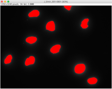       Example of thresholding cell nuclei using ImageJ
     • Check the box for "Dark Background".
     • Click on the "Set" button and type in your threshold values (use 65535 for the upper threshold level).
   • Go to Process -> Binary -> Make Binary.
     • This makes the image black and white, where the white areas should correspond to nuclei locations.
3. Use the newly created image to count cells.
4. Run the analysis by selecting Analyze -> Analyze Particles.
   

   

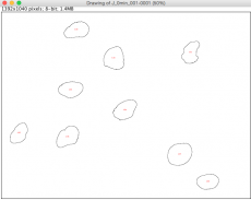   Example of areas identified by intensity thresholds for DAPI channel in ImageJ
   • In the "Size" field, type 200-Infinity. This will eliminate small, extraneous particles that do not correspond to nuclei.
   • "Circularity" can remain at default values: 0-1.
   • "Show" should say "Outlines". This will allow you to manually assess the quantification.
   • Click the following options: Display results, Exclude on edges, Summarize.
   • Press OK to complete.
5. A window will pop up showing outlines of each nucleus the software identified based on the thresholds you defined. Each identified area is labeled with a red number, corresponding to the left column of the data shown in the "Results" window.
6. Take a look at the "Results" window to see the results of the analysis. It is good practice to validate the numerical results by comparing them to what you see in the images.
   • Do the outlines correspond to all nuclei seen in the image?
7. Copy the count number from the "Results" window into your lab notebook for each image.
8. Normalize the total FITC intensity across images and experimental groups by dividing the intensity by cell number as determined by nuclei number.
9. Record this data in your notebook. We will use statistics to assess any differences between experimental groups on M2D8.

In your laboratory notebook, complete the following:

• Do your qualitative assessment of the expression data and rough quantitative data analysis match up?
• What experiments could you do to either reconcile differences between the data or follow up to get more information about expression of your Fet4_mutant?

Reagents list

• Synthetic dropout - uracil (SD-U) media: 0.17% yeast nitrogen base without amino acid and ammonium sulfate (BD Bacto), 0.5% ammonium sulfate (Sigma), 0.192 % amino acid mix lacking uracil (Sigma), 2% glucose (BD Bacto), 0.1% adenine hemisulfate (Sigma)
• Synthetic dropout - raffinose (SD-R) media: 0.17% yeast nitrogen base without amino acid and ammonium sulfate (BD Bacto), 0.5% ammonium sulfate (Sigma), 0.192 % amino acid mix lacking uracil (Sigma), 2% raffinose (Sigma), 0.1% adenine hemisulfate (Sigma)
• Synthetic dropout - galactose (SD-G) media: 0.17% yeast nitrogen base without amino acid and ammonium sulfate (BD Bacto), 0.5% ammonium sulfate (Sigma), 0.192 % amino acid mix lacking uracil (Sigma), 2% raffinose (Sigma), 2% galactose (Sigma), 0.1% adenine hemisulfate (Sigma)
• Cadmium chloride (Sigma), stock concentration= 100mM
• Iron chloride (Sigma), stock concentration= 100mM
• ULTREX II, Ultrapure Nitric acid (J.T. Baker)
• Hydrophilic PTFE 0.22μm filters (J.T. Baker)
• Metal-Free sterile polypropylene tubes (VWR)

Navigation links

Next day: Analyze ICP-OES data and examine yeast tolerance to metal

Previous day: Immunofluorescence staining