20.109(S18):Analyze small microarray data (Day3)

Introduction

In this module, you will build upon the research completed by former 109ers. Using the results of their small molecule microarray (SMM) you will complete secondary assays to confirm the binders identified. Today you will use the data previously collected to identify 'hits', or ligands, that are able to bind FKBP12. Though you may be able to qualitatively visualize spots that appear to emit more fluorescence, it is important to complete quantitative analysis that supports your observations.

In Spring 2017, the class used microarrayer to read the fluorescence signals on the surface of the SMM at two excitation wavelengths. As noted previously, the 532 nm wavelength was used to excite fluorescein, which was printed in an 'X' pattern to assist with alignment. The 635 nm wavelength was used to excite the fluorophore-conjugated anti-His antibody, which should only bind FKBP12. A hit denotes a spot on the slide that emits a fluorescence signal significantly higher than the background fluorescence level. In terms of protein binding, a hit denotes that the FKBP12 protein is bound to a compound and the antibody is therefore localized to that position on the slide. You will analyze the fluorescence emission data collected by the microarray scanner using two quantitative approaches: a robust z score.

When the Koehler Lab prepared each printed glass slide, the microarrayer also produced a GAL file, or GenePix Array List, which can be viewed using Excel. The GAL file contains information about where each spot was printed, and what compound was printed there. However, the relationship between the GAL file and the actual contact of the print head is very imprecise. Instead, we will use the fluorescein guide spots to align the array in the GAL file to the true print location for each pin. For this alignment, we’ll use a tool provided by the Chemical Genetics Section at the NCI. This tool searches the scanned image for these guide spots and attempts to rotate, translate, and scale the array to best match the observed fluorescence. Following the alignment, we will compare the fluorescence at 635 nm within the deposition region of each spot (foreground) to the fluorescence immediately outside of this region, where nothing was printed (background). We’ll use these values to calculate a robust z score. From the robust z score, we can determine the associated probability that the observed fluorescence occurred by chance, and if this probability is sufficiently low, we call the compound a hit.

(Written with assistance from Rob Wilson, graduate student in the Koehler Laboratory.)

Protocols

Part 1: BE Communication Lab workshop

Our communication instructors, Dr. Sean Clarke and Dr. Prerna Bhargava, will join us today for a workshop on crafting clear and informative figures with captions.

Part 2: Align the array and quantify spot fluorescence

The SMM alignment tool is provided on 20.109 laboratory computers. If you feel comfortable working with a Python development environment, we can also make the source code available to download. This will require the installation of Python 3.5 and multiple third party libraries which are included in Anaconda 4.2.0.

1. Download the .tiff files (in the table assigned by team section / color) and .gal files (in the link above the table) that correspond to the barcodes your team is assigned on the Class data page.
2. Download on the desktop of your 20.109 computer this software package, developed by Rob Wilson and courtesy of the NCI Chemical Genetics Section.
3. Open a Terminal window from Finder\ Applications. Type in python ~/Downloads/SMMAnalysisTool, and press Enter to execute the code.
   • Note: a recurring bug may prevent the menu bar from responding. If this occurs, click out of the window then click back into the window.
4. Open the .tiff file for one of your slides by selecting File → Load TIFF.
   • These files should be in the Download folder.
   • You can change the wavelength channel that is displayed using the drop-down menu labeled 'Display'.
   • You can adjust the background fluorescence signal by moving the top slider rightward.
   • You can saturate the foreground fluorescence signal by moving the bottom slider leftward.
5. Visually inspect the slide image and note all observations concerning flaws (damaged spots), obvious hits, residual fluorescence, etc.
6. Open the .gal file corresponding to the barcode on the slide by selecting File → Load GAL.
   • Note: the GAL file for each slide is specific to that slide and you will therefore need a different GAL file for each slide.
   • Hover your cursor over the interesting spots observed to see which compounds were printed at these locations.
7. In the box labeled 'Guide Name' at the left of the window, type "Sentinel" in the field for 532.
   • Leave the field for 635 blank as we do not use guide spots in this channel.
   • You should observe spots in the array turn green in an X pattern (the pattern in which the fluorescein spots were printed).
8. Click the 'Align All' button at the lower left of the window to align the entire array to the nearest observed guide spots.
   • Confirm that the alignment is reasonable throughout the entire slide.
   • Flaws in the slide may disrupt the alignment and negatively affect the quantification.
9. Click the 'Align Each' button at the lower left of the window to align each subarray to the nearest guide spots.
   • Confirm that the alignment is reasonable for each block.
   • If the alignment is not reasonable, or can be improved upon, you should drag and drop the spot outlines manually.
   • To return to the original array, click the 'Reset' button at the lower left of the window.
10. Select File → Save Image to save a picture of your slide.
    • This saves the current channel exactly as it is displayed in PNG format.
11. Calculate and save the fluorescence of the foregrounds and backgrounds of each spot.
    • Select File → Save Spot Intensities.
    • This will output a CSV file.
12. Repeat Steps #4-11 for each of your slides.

Part 3: Calculate robust z scores and call hits

The output data, or CSV, file you created in Part 1 saves the information for each spot on your SMM. Each spot contains one compound and each compound was printed at multiple spot locations. Ultimately, we are interested in the summary information for each compound that was printed on your slides. To analyze the summary information, we will use a Pivot Table. A Pivot Table is a data summarization tool that is able to sort, count, total, or average the data stored in one table or spreadsheet. This tool allows researchers to quickly highlight and manipulate desired information within more complex spreadsheets. You will use a Pivot Table to calculate the z scores for your data.

The directions below are written according for use with the 20.109 laboratory computers. If you use your own computer, the directions may be slightly different, especially if you use a PC. Please ask if you need assistance!

1. Open the output data CSV file for one of your slides in Excel.
   • There are several columns, but don't worry; we are only interested in the one labeled 'SNR 635'.
   • This value represents the signal-to-noise ratio calculated in the 635 nm channel and is defined by SNR = ( μ_foreground - μ_background ) / σ_background , where μ is mean and σ is standard deviation.
     

     
2. Select Data → Summarize with PivotTable to summarize the data and create a PivotTable in a new worksheet.
   • Be sure that a cell within your spreadsheet is highlighted (any cell will work).
   • A new Sheet will be created in your spreadsheet and the 'PivotTable Builder' window should appear.
3. To populate your PivotTable complete the following:
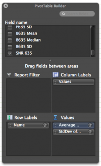
   • From the 'Field Name' box, select 'Name' and drag it into the 'Rows' box.
   • From the 'Field Name' box, select 'SNR 635' and drag it into the 'Values' box.
     • Excel will default to 'Sum' of SNR635. Change to 'Average...' by clicking the i then selecting Average from the 'Summarize by:' options.
   • Again, from the 'Field Name' box, select 'SNR 635' and drag it into the 'Values' box.
     • Change to 'StdDev...' by clicking the i then selecting StdDev from the 'Summarize by:' options.
   • Be sure your 'PivotTable Builder' window looks like the image to the right.
4. The PivotTable should be populated as you complete the items in Step #3 and appear similar to the image below. When you are done, close the PivotTable Builder window.
   

   
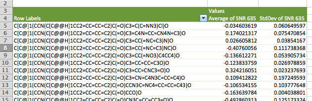
5. Calculate the median absolute deviation, defined as MAD = median ( |x_i - median(x)| ).
   • Enter "=MEDIAN(ABS(data-MEDIAN(data)))" where data is the data range in the 'Average of SNR 635' column.
   • If the value does not appear: After you enter the equation, click within the fx field and use the key stroke 'COMMAND + SHIFT + ENTER' to input the array formula.
6. Calculate the robust z score for each compound, defined as Z = (x_i - median(x)) / (1.486(MAD)).
   • Enter "=(cell-MEDIAN($data))/(1.486*$mad) where cell is the cell containing the 'Average of SNR 635' for the compound, data is the data range in the 'Average of SNR 635' column, and mad is the fixed value in the cell that contains the calculated MAD.
   • Time-saving tip: After you calculate the z score of the first compound, double-click on the small black box at the bottom right of its cell; it will automatically expand the formula to all available rows!
   • If you have trouble calculating the Z-scores, an alternative approach can be used:
   1. Copy the Pivot table as values to a new sheet
   2. Create a column named "Abs difference to median" to calculate the absolute difference between data points and the median. Type in the formula "=ABS(data point - MEDIAN(data column)" where data point is a single entry in the "Average of SNR 635 column" and data column is all the entries in the "Average of SNR 635" column. Use the time-saving tip above to fill all rows for the column.
   3. Calculate the MAD as "=MEDIAN(Abs difference to median column)"
   4. Proceed to calculate the Z-scores as above
7. Sort your compounds by robust z score.
   • If you chose not to use the Pivot Table, you can sort the Z-scores by first selecting all columns except the column with the MAD value (make sure this value is in the rightmost column as sorted columns need to be adjacent to each other). With the columns selected, go to the data tab and click on sort. Set the column to be the column holding the Z-scores and the order to be Largest to smallest. Click OK. Be aware that if you select the column holding the MAD value.
8. In the next column, you will indicate which compounds are common binders and thus are not necessarily specific to the protein of interest.
   • Download this Excel spreadsheet into the same folder as the other CSV files output by the SMM data analysis software. This spreadsheet categorizes whether certain compounds should be included or excluded in your results. Compounds are excluded if they are known to bind to two or more different proteins.
   • In the next column of your CSV data analysis file, enter "=VLOOKUP(firstcell, '[Specificity2.xlsx]Specificity'!$A$2:$W$50001, 23, FALSE)" where firstcell is the cell address containing the first compound SMILE.
   • Expand the formula to all the available rows.
     • If the entry states "exclude," the corresponding compound is a common binder and should be excluded from your results.
     • If the entry states "include" or "N/A" (meaning that the compound was not in the spreadsheet of potential binders), then include these compounds in your results.
9. Email the list of hits identified in your analysis to the teaching faculty.

Part 4: Choose ligand hits for secondary assays

1. The teaching faculty compiled a list of all of the ligand hits identified from all of the slides used in the Spring 2017 screen (linked here). Each team will select two ligands to assess in secondary assays: one testing protein activity and one confirming ligand binding. Sign-up on the sheet at the front laboratory bench when you decide on your ligands.
2. To visualize the structures of the selected ligand hits, open ChemDraw on the 20.109 laptop computer.
   • Copy the SMILES of the compounds (from column F of the Excel spreadsheet attached to Step #1).
3. In ChemDraw, go to Edit/ Paste Special... and choose SMILES.
   • You can now visualize the chemical structure of the hits with high resolution, and save this image for your Data Summary.

Team (T/R section)	Ligand #1	Ligand #2	Team (W/F section)	Ligand #1	Ligand #2
Red			Red
Orange			Orange
Yellow			Yellow
Green			Green
Blue			Blue
Pink			Pink
Purple			Grey
White
Grey

Navigation links

Next day: Evaluate protein purity and concentration

Previous day: Purify protein for secondary assays