20.109(F11): Mod 2 Day 2 Measuring system performance

Measuring System Performance

Introduction

In designing a synthetic biological system it can be helpful (to you and to others) to describe the system using a high level design language that can simplify or "abstract" what's going on with the system. For example the bacterial photography system might be depicted as two key devices, one device that detects a signal and a second device that generates an output upon receiving information from the first device. Such a ���black box��� depiction of the system's operation enables easy re-use of the devices by others as well as helpful specifications for the needed connections between the devices (versus the materials needed for operation within them). For example, light is the input for the bacterial photography system, but it's straightforward to retask the system as a chemical sensor instead: just swap out the first "input sensing device" from one that's sensitive to light to one that's sensitive to your chemical of interest. Similarly, the output of the bacterial photography system is a black colored product but imagine hooking up the light sensing input device to chemotaxis as the output...then the cells might swim to the light rather than turn a color in response.

"Black box" depiction of bacterial photography system

Operation of System's Devices

In this module we will not be re-designing the system but rather tuning it to increase the dynamic range. Thus we'll have to look carefully inside the "black box" depictions of the devices and in this way become "device experts" rather than "system experts"--though a clear understanding of the system we're working with is obviously needed. To look in the black box that senses light, we'll have to learn more about the two component signaling cascades that the device is built from.

Two Component Signaling

As was mentioned last time, the bacterial photography system exploits a common signaling pathway in prokaryotic organisms, namely the "two component signaling" (2CS) pathway. As you learned, the two components are the sensor and the responder molecules and they are sensitive to changing environmental conditions. Hundreds of signaling pairs have been identified, and though variations are plenty, there is a common theme to the signaling mechanism the two components use. In general the communication of the 2CS pair is via a three reaction "phosphorelay."

Rxn 1: ATP + Sensor_His --> ADP + Sensor_His~P

Stimulation of the sensor by a ligand (or a change in the environment or a detectable cellular input) leads to a change of state for the sensor, e.g. it may dimerize, change conformation, etc. This altered state stimulates the autophosphorylation activity of the sensor and the gamma-phosphate from ATP is transferred to a histidine on the cytoplasmic face of the sensor. Thus another name for the sensor molecule is "histidine protein kinase" and when a number of sensor molecules are compared, the histidine that is phosphorylated can be identified based on conserved sequence motifs that surround it.

Rxn 2: Sensor_His~P + Responder^Asp --> Sensor_His + Responder^Asp~P

To transduce the signal from the sensor that's at the membrane to an effector molecule within the cell, the phosphate on the conserved histidine of the sensor is transferred to an aspartate molecule on the responder. The phosphorylation state of the responder regulates its activity. In many cases, the phosphorylated aspartate enables the responder to bind the DNA and regulate relevant genes, provoking a sensible cellular response to the initial stimulus, e.g. swimming to the good food, transcribing pores to let in ions, etc.

Rxn 3: Responder^Asp~P + Sensor + H₂O --> Responder^Asp + Sensor + P_i

To reset the signaling system, the phosphorylation state of the regulator must be returned to its original set point. A phosphatase activity is associated with many of the sensor molecules in 2CS paths, enabling a single molecule to both enhance and diminish the signaling, consequently provoking and dampening the necessary response.

Inside the black box abstractions

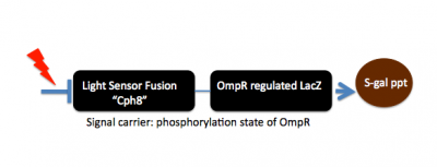
The bacterial photography system we are studying modifies a natural osmolarity signaling pathway in E. coli so that light striking the cell can be converted to a detectable output. The green and orange dumbell-shaped cartoon in the figure (below) represents the input sensor. It's represented as a dumbell since light-sensing requires the combined action of two proteins: a natural light-sensing protein called Cph1 that comes from an algae (shown as the green lobe) and the transmembrane two component signaling protein called EnvZ (shown as the orange lobe). To fully function, the cell must also express phycobilin producing proteins to make accessory pigments needed for the light-sensing fusion protein to work. These phycobillins are shown in the box at the left of the signaling pathway and marked as "PCB" on the green lobe of the fusion protein cartoon. The Cph1:EnvZ fusion, called Cph8 by the authors of the paper, starts a phosphorelay within the cell���s osmoregulation pathway. OmpR is the response regulator and signal carrier, changing the activity of an OmpR regulated promoter that is directing transcription of LacZ. Finally the ��-galactosidase enzyme from LacZ works on a chromogenic substance, Sgal, turning the media dark when LacZ transcription is high (i.e. cells are grown in the dark) or precipitating less color in the media when LacZ transcription is low (i.e. cells are grown in the light)

Returning to the generic "black box" description of the system, we can fill in a few of the details, in a way that emphasizes the device details and aspects that might be manipulated to tune the existing system. You can decide for yourself if this is a helpful depiction of the system. Remember that you would like to have an image that emphasizes means of tuning the system. In our experiment, we'll be focusing on the OmpR signal carrier between the two devices. There are other ways to affect the input and output responses though and you should consider how helpful (or not) this abstraction is. If you like the depiction of the system shown here, know why. If you don't, come up with a better one!

Details inside of bacterial photography system

Today, we will assess the bacterial photography system as it was originally made. We'll measure enzymatic activity as well as view the resulting bacterial photograph. Next time we'll start to "tune" the system in order to expand the dynamic range of the system.

Protocols

Part 1: ��-galactosidase assay

You should perform assays on your overnight liquid cultures that were grown in the dark and the light. Refer back to the protocol from day 1. Activity calculations for today's samples will be part of your assignment for next time.

Part 2: Black and white photography

Retrieve the Petri dishes you set up last time and compare the appearance of the light and dark grown samples. Because the dark grown cells were in a completely dark box, the difference between the two plates reveals the greatest contrast you can expect in your bacterial photographs. You should take a photograph (digital!) of these petri dishes since the result will be included in the final research article you write for this module.

Next decide what image you would like to develop as a bacterial photograph. Generate a computer file with this image and print it to a transparency. Transparencies will be available in the lab for you to use as masks. As you choose an image, remember that the goal is to have each cell growing distinctly in the light or dark. Remember that light can bounce around edges and may blur the resulting image if the black and white are highly intermingled. In general, it���s better to have a dark background and a light image rather than the other way around. To darken the dark parts of your photo, you might want to print it on two transparencies and use them both to mask your Petri dish.

Media containing S-gal is available for you to supplement with antibiotics and cells as you did last time. Once you've supplemented and poured a plate, let it solidify ~30 minutes at room temperature then tape the transparency to the back of the dish. Place your bacterial photograph in the 37�� incubator (media side up) and when the class is ready, we'll turn on the red-lamp to expose the "coliroids" until next time. You will want to adjust the placement of the dish in the incubator once the light is on. The rule of thumb is the light image on the plate should be clearly visible but not super bright. If you can see the image clearly, and it doesn't look dim, you're probably in the right range.

Part 3: CAD Tool for Synthetic Biology

Computer-aided design (CAD) is a hallmark of several mature engineering disciplines, like mechanical engineering or civil engineering. These engineers can rely on computer simulations to reliably predict the behavior of a car or a bridge, rather than run a hundred cars into walls to see how they perform. Biological engineers have fewer good CAD tools at their disposal. More often, they must run laboratory experiments to test a system. But wouldn't it be nice (and quicker and less expensive too!) to try a few things on a computer first? And then, with some good candidate designs in hand, we could turn to the bench with more confidence, having eliminated the clear failures.

Tinkercell

One early effort at a CAD tool for synthetic biology is TinkerCell, developed by engineers at the University of Washington. TinkerCell allows you to visually construct and then simulate/analyze a biological network. Using the following instructions, you can use TinkerCell to build the bacterial photography system (or at least a simplified model of it). For those who would like to read more about the TinkerCell CAD tool, you can find the details in this article from the Journal of Biological Engineering.

Get started!

Open the TinkerCell application that has been loaded onto the laptops in the lab (do not download an updated version of the program if you are given that option!). The instructions in this tutorial were written for the Mac-based version of the program (1.2.472). If you are running a different version of TinkerCell or if you are running Tinkercell on Windows or Linux, you may see some subtle differences.
After you open the TinkerCell application, begin familiarizing yourself with the basic operation of the program. In particular, try to use

• the Molecules and Reaction tabs: try to select 2 molecules from the molecules that are available. For example, click the "Enzyme" on the icon strip and then click the network canvas to place an enzyme. Repeat with a second molecule, selecting "Transcription Factor" from the icon strip and placing it on the network canvas. Next, choose the Reaction tab and select either activation or repression. Click on the enzyme first, then the transcription factor. If you chose activation, you'll be asked to choose between two mechanisms. A reaction arrow should appear. Next, if you like, try stamping out two receptor molecules and connect them with a different kind of regulation, or try making an enzyme catalyze a reaction with one or more small molecules.

• the Parts and Regulation tabs: Choose the Parts tab and try stamping out a gene expression cassette, i.e. an operator (activator or repressor binding site), a promoter, an RBS, a protein coding sequence, and a terminator (optional). The parts do not need to be aligned when you place them on the network canvas, but if you drag them next to one another they should connect. You can then choose "Transcription Regulation" from the Regulation tab, and link the transcription factor you placed earlier to the gene's operator. A reaction arrow should appear. You can move the icons on the canvas, reshape the reaction arrows, and relabel the parts to your liking. Try using "Protein Production" from the Reaction tab to make the coding region of the gene produce a protein.

Building the bacterial photography system

Fully built bacterial photography system

Now that you have the basic mechanics in hand, you can build the bacterial photography system. Follow the steps below.

• Start this project on a new canvas. Select "New Canvas" from the File Menu, or click the new page icon on the top toolbar.
• Assemble the reporter gene: From the "Parts" tab, place an "Activator Binding Site", "Promoter," "RBS," and "Coding" icon on your canvas. Drag the parts next to each other, in that order, so they snap together.
• Name the reporter gene elements: Click on the name below each part to rename it. The promoter should be named "PompC." The RBS can be left as is. The coding sequence can be renamed "LacZ".
• Add the transcription factor: From the "Molecules" tab, select "Transcription Factor" and place one on the canvas. It will represent the phosphorylated form of OmpR, so rename it "OmpRp".
• Visual appeal: Select the OmpRp protein, and then from the "Edit" menu choose "Add decorator." A dialog box will display a choice of icons. From the "Decorators" tab, select "phosphorylation".

Regulating transcription

• Activate Transcription of PompC with OmpRp: From the "Regulation" tab, choose "Transcriptional Activation" and then click on OmpRp and the activator binding site just before PompC. Choose ���Transcription Activation��� from the pop-up menu.
• Add the Cph8 light receptor: From the "Molecules" tab, choose "Receptor" and place one on the canvas. Rename it "Cph8."
• Regulate OmpRp with Cph8: From the "Regulation" tab, choose "Allosteric Inhibition" and then click on Cph8 and OmpRp. You can reshape the regulatory arrows and move the elements around the canvas as needed for clarity.
• Add the Beta-Gal protein: From the "Molecules" tab, place an enzyme on the canvas and call it "BetaGal". Link it to the LacZ coding region using the "Protein Production" reaction.
• Add the colorful small molecule: Place two more small molecules on the canvas. Connect them to your BetaGal protein using "Enzyme Catalysis" from the "Regulation" tab. Name the input molecule "SGal", and the output molecule "COLOR." Next, double-click on SGal to open a dialog box. Select the "Initial Conditions" tab and increase the concentration to 15.
• Add a Chassis: From the "Compartments" tab, choose ���Cell��� and place one on the canvas. Move and resize the cell so it encloses the transcription factor and the reporter gene. Leave the Cph8 receptor in the cell membrane.
• Add light: From the "Molecules" tab, choose "Small Molecule" and print one on the canvas. Rename it "Light" and connect it to Cph8 with an activation arrow from the "Reaction" tab.
• Turn the light on: From the "Inputs" tab, choose "Step input" and click on the Light molecule. Next, find the cell compartment in the "Model Summary" list of components on the right. Click the arrow to expand its subcomponents, find the Light molecule, and expand it. Change the value of "step_time" to 50 (this will turn on the light halfway through the simulation, rather than right at the beginning).

Whew!

Now that you've dragged, dropped and connected all the parts in the bacterial photography system, it's time to consider what you've got. Did you learn more about the system by building it? Can you see places where different parts might be interesting to try? How big is the gap between the things we know about, and the things we need to learn more about? Are there any experiments you'd like to try? What reactions could you measure? What could you mutate to improve?

Simulating the bacterial photography system

Simulation output

Behind the shiny-looking front end of TinkerCell is some serious mathematical capability. We'll use the "Deterministic" simulator (i.e. we will be ignoring the random fluctuations that would occur in a real cell). Click the big green arrow in the top toolbar to run the system.

You should see a graph window and a second window with sliders. To make the output a little easier to read, click on "Legend" in the graph window, and uncheck everything except Time, Light, Cph8, OmpRp, LacZ, BetaGal, and COLOR. Take a few minutes to familiarize yourself with the output graph.

Tuning the system

Turn to the slider window and start changing numbers, making notes of what effects you see. Remember that if the system's behavior gets way out of whack, you can always close the graph/slider windows and re-run the simulation with default values. Many of the variables in the slider window have straightforward names, like "light_step_height", but some are more opaque. In general, things named "Kd" are constants governing the strength of a regulatory interaction. "Kcat" is the catalytic efficiency of the BetaGal enzyme.

Tweaking the system

Use this model to realize a design specification you have in mind. First, you must decide on some specific changes you would like to make to the system. Here are some possibilities:

• Change the amount of SGal in the bacteria's environment (the "cel1_SGal" slider). What happens to the COLOR output?
• Change the efficiency of the BetaGal enzyme (the "cel1_ec1_Kcat" slider). What happens to the output?
• Decrease "Light_step_steepness", so that the light turns on gradually rather than all at once. Does this tell you more about how exactly the system responds when its input changes?
• Try changing the light's step input to a sine wave input, and change the frequency. What happens to the output when the frequency is high? When the frequency is low?
  

Next, you can tinker with the outputs. Would you like the bacterial photographs to develop faster/slower/darker/lighter...? What change would be needed to affect the simulation and the graph in that way. See if you can find the right combination of sliders to make those changes happen. Here are some ideas:

• the bacterial photographs require at least 24 hours to develop in the lab, but they are stable once formed. What elements in the system could be changed to make the COLOR output accumulate more slowly? More quickly?
• the bacterial photographs can sometimes look less intensely colored than the original mask that's used to generate the image. What elements in the system could be varied to change the total amount of color produced?

Part 4: Instruction on Oral Presentations

Over the course of the term, everyone taking 20.109 will be making two presentations to the class. One will be a presentation of a primary journal article related to either 2 component signaling systems or synthetic biology. The other presentation will be of a research idea. Today our wonderful coaches from the Writing Program will come to lab to give a talk about giving talks. This presentation should be a welcomed chance to learn what's expected when you speak (in 20.109 and elsewhere) and to gather some great tips for giving polished and interesting seminars. You can follow up this instruction by re-reading the | oral presentation guidelines we've assembled for this subject.

DONE!

For Next Time

1. Calculate the units associated with the bacterial photography system grown in the light and the dark. Use this data and the photographs of your petri dishes grown in the light and the dark to draft Figure 1 of the research article you'll write for this module. Be sure this figure has all the traditional elements for figures (title, legend, labels etc).
2. Consider again the depictions of the photography system that we've looked at (system level depictions, biology cartoon, device level operation). In particular, think about how you might use the image below to describe the experiment you'll be doing. Is there a better depiction for the system and the aspects of it that you'll be manipulating? If not, say why. If so, sketch it out and say how it's better. There's no "right" or "wrong" here but it's important to think about effective figures that summarize and anticipate your work.
   

   

Reagents

See Mod 2 Day 1.