Difference between revisions of "Spring 2020 Assignment 8"
From Course Wiki
(→Fourier transform table) |
|||
| Line 61: | Line 61: | ||
</center> | </center> | ||
| − | |||
| − | |||
| − | |||
| − | |||
| − | |||
| − | |||
| − | |||
| − | |||
| − | |||
{{Template: 20.309 bottom}} | {{Template: 20.309 bottom}} | ||
Revision as of 15:19, 24 April 2020

Circuit analogies
| |
For each of the systems below, find an analogous circuit. |
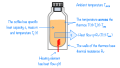
Thermal system:Coffee in a thermos
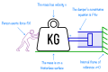
Mechanical system: mass and damper


Convolution practice
| |
For each of the pairs of functions below, plot the convolution of the two functions, $ Y=A*B $ |
| $ A $ | $ B $ | $ Y=A*B $ |
|---|---|---|
%2Bdelta(t-1).png)
|
|

|
|
|

|
|
|
|

|
|
|
|
|
|
|
|

|
|
.png)
|
|
|
Fourier transform table
The two tables below show important properties of the Fourier transform and several useful transform pairs. You can use the tables of pairs and properties to figure out the transforms of an endless number of functions.
| |
</div> |

