Spring 2012:Leanna Morinishi Lab 1

Lab 1: Optical Trapping

Goals

We set out to add functionality to the trap control software, specifically we wanted to automate centering of the DNA-tethered bead using a centering algorithm which we would write in MATLAB. To center the DNA-tethered bead we would need to learn how to communicate with different electronics using DAQ and the daqtoolbox in MATLAB, how to test a code which is supposed to provide specific functionality, and a bit about the UI in MATLAB. Beyond this, we tried to:

• Get nicer calibration data
• Look at the properties of the tether, to calculate the persistence and contour lengths

Skills Learned

• How to talk to the DAQ and ActiveX controls
• More about QPD and piezo-electric
• How to put a button on a UI in Matlab!!

Methodology

Materials and Instruments

• Matlab: programming language
• DAQ
• Piezoelectric Stages
• Bead size: 0.97 um beads used
• Laser wavelength: λ = 975 nm

Centering Function

• First, I learned how to activate channels, and talk to the DAQ
• I then created a sine wave and had it repeat infinitely, then acquired that same data from the DAQ

• At its most basic level, our centering function:
  • Establishes a waveform in the x-direction, calculating the center position
    • Repeat in y-direction
  • Move the stage to the calculated center position

• It calculates the center position in each direction by
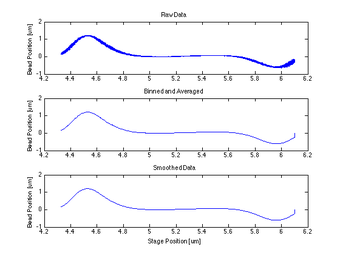
  • Binning and averaging the QPD and stage data from the sinusoid
  • Smoothing averaged data
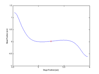
  • Finding the indices of the max and min and taking the information at the median point between them to calculate the center position relative to the current stage position
  • Establishing a new waveform using the newly calculated center position

• See Code Section for more details

Estimating contour and persistence lengths

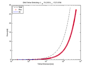
The worm-like chain model is one method to approximate the behavior of DNA when stretched. Here we are interested in the extension curve of a DNA tether, so that we may use its (hypothetically) linear region to calculate the place of tether attachment. We fitted our data (guided by calibration calculations) to the following model equation using nlinfit to solve for the persistence and contour lengths.

$ F = \frac{k_{B}T}{l_{p}}[(\frac{1}{4}(1 - \frac{x}{l_{c}})^{-2} - \frac{1}{4} +\frac{x}{l_{c}}] $

where $ k_{B} $ is the Boltzmann constant, $ x $ is the end-to-end distance of the DNA, $ T $ is the temperature, $ l_{c} $ is the contour length and $ l_{p} $ is the persistence length.

Calibration Coefficients

Past attempts at calibration yielded these values, which were used in the extension curve fit. (While values were found using the PSD method outlined in the 20.309 lab manual with n=14, 18, 16 at V=30, 60, 90 mW, they failed to follow a consistent logical progression, and therefore should be taken with a grain of salt. We tried using other data - from past years and this semester - to glean better results, to no avail.)

	Stage um/V	QPD Sensitivity V/um			Trap Stiffness N/m
Power mW	All	20	70	120	20	70	120
Values	2.22	0.5	1.75	3.0	5e-5	1.4e-4	2.4e-4

Results

Force/Stretching Estimation using nlinfit

Figure 1. A force extension graph showing the raw and fit data with the ideal. Calculated the contour and persistence lengths using data collected in a 20mW trap while the sample underwent sinusoidal oscillation in the y-direction.

	nlinfit Values [nm]
	20 mW X	20 mW Y	70 mW X	70 mW Y	120 mW X	120 mW Y
$ l_p $	71.42	70.24	68.65	91.43	68.28	79.70
$ l_c $	1698.40	1727.08	1766.89	1332.48	1776.45	1521.90

• Mean fit values:
  • $ l_p $: 74.95 ± 9.08 (std)
  • $ l_c $: 1637.2 ± 175.60 (std)

Proof of Concept for Center Calculation

The following data is one example, taken from tethered bead data at 20 mW. This method will work best with a tethered bead stuck in the trap at an oscillation amplitude > the length of the tether.

Figure 2. (1) shows the raw QPD data taken from a sample undergoing a continuous sinusoidal wave in the x-direction while in trap at 20mW, (2) shows QPD data binned and averaged data, and (3) shows the smoothed binned data.

Figure 3. Smoothed data from Figure 2 cut off at the max and min, and the center is calculated by finding the median index (red), against strain gauge voltage.

Plotting the Centering Calculation on OTKB GUI

Figure 4. This is an example of the GUI while the function calculates the center of the trap in the y-direction. Calculated centers are marked by a X.

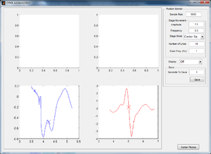
While the stage moves in a single sinusoid in the x-direction and y-direction, the data and calculated center are plotted on the GUI for visual confirmation of working data. The left graph shows the x-direction QPD detected movement and calculated center, and the right graph shows the y-direction movement and center. In Figure 4, the stage has just moved in the y-direction and therefore the curve in the y-direction looks clean while that in the x is close to zero and inconsistent.

Discussion

Force Extension Curve

• We originally did this fit because

1. Steven Nagle said so
2. This method may have helped us find the tether center if we were to fit the linear portion of the force-displacement curve.

• However, we ended up not going down this path. Still, we report our findings here.

• Here, nlinfit found similar measurements of $ l_{p} $ and $ l_{c} $ for most of the samples, and while the averages have the same order of magnitude as the expected values, they are not within the calculated standard deviation.
  • Accepted Values: $ l_{p} $~45nm and $ l_{c} $~1180nm
  • Calculated Values
    • $ l_p $: 74.95 ± 9.08 (std)
    • $ l_c $: 1637.2 ± 175.60 (std)
• This might be due to poor calibration values (listed above). However, the function was most sensitive to the V/um calculated conversion factor of the QPD voltage (0.5 V/um in the code), and even when changed two orders of magnitude in either direction, the $ l_{p} $ and $ l_{c} $ values did not vary an order of magnitude.
• We noticed that our function did not have variables that accounted for linear displacement in the F or x directions. We added these to the function, together and individually. In all cases nlinfit spat them back and said that the function was insensitive to these new parameters.
• The data indicates that our DNA tether persistence and contour lengths are 1.66 and 1.38 times the given lengths, respectively. Why? Dunno. Speculate.

Tether Centering

Conclusion

Code

You can view the functions on my Public until ~June 2012.

OTKB

Main DNA Tether Centering Function (Wasserman)

Matlab GUI

We took this code from Steve Wasserman and tweaked it to include our function.

• First we altered this line in the OTKB OpeningFcn to add our option to the popup menu on the gui.
  • set(handles.popupmenuStageMovementMode, 'String', {'Off', 'X', 'Y', 'XY Scan', 'Hypocycloid', 'Center Sample'});
• Within StartQpdMonitor, and within the cases we added another few lines of code which do the following if the popup menu is set to 'Center Sample'
  • It calls our function DNATetherCentering, with the handles and the user interface settings as inputs
  • The function outputs two values: the x and y voltage values of the tether center
  • The new waveform is established as the x and y location mentioned above
  • The popup menu is then reset to 'Off' and the StartQpdMonitor function continues on to place the new waveform in the daq output buffer and then implement it as the output

DNATetherCentering

Find DNA Tether Center Function

• Takes in handles (struct that contains handles and user data) and UiSettings (struct that contains current user defined settings)
• The function cycles through thrice
  • If it is the first cycle, many basic settings are established or pulled from the handles or UiSettings, such as the SamplesToSave, the amplitude, time, and frequency of the oscillation, the numberOfSamples in time, the SampleRate, and the shape of the initial waveform.
  • We established the SamplesPerTrigger to record as 1.5*numberOfSamples because we want to ensure that we collect the entirety of the waveform
  • We start the input channel
  • We put the current waveform into the output buffer (if 1st cycle, set to 1 sine wave in the x direction, 0s in the y direction)
  • We start the output channel
  • We trigger the input then the output channel with manual triggers
  • We gather data from the input with getdata
  • We stop both channels
  • We run the findCenter function which calculates the center in the given direction
  • We plot the binned data from findCenter and the calculated centers on the gui
  • After three cycles, the function returns the calculated x and y center voltage values of the stage

• findCenter
  • This function begins by taking the recorded Qpd data and binning it based on the associated strain gauge voltage data in both the x and y directions
  • The currentPositionX and Y are set as the final value of the collected data in strain gauge voltage
  • Then the maximum and minimum Qpd value indexes are calculated for both X and Y directions, and the median index is found and established as the centeredPositionIndex
  • If this is the 1st cycle
    • The CenterPositionX is defined as the previous stage location, plus the binned Qpd value at the centeredPositionIndex in X, minus the currentPositionX defined earlier
    • The new waveform is defined as a single sine wave centered at the previous stage location in the y-direction, and a constant voltage value of CenterPositionX in the x direction
  • If this is the 2nd cycle
    • The same as the 1st cycle, except you are calculating the CenterPositionY, and the new waveform is a sine wave transposed by CenterPositionX in the x direction and a constant value of CenterPositionY in the y

persistenceLength

Calculate persistence and contour lengths by nlinfit

• Defines constants
  • Temperature at 293K
  • l_p0 and l_c0 as the guesses for the persistence contour lengths respectively
• Takes in data from a .txt file of a DNA tether sample, could be any file
• Converts the QPD and strain gauge voltage data into um using a known conversion factor 2.22 um/V for the strain gauge and .5 V/um from calibration coefficients calculated in 20.309 last semester
• Defines 1000 edges of the bins using linspace between the min and max values of the strain gauge data
• Uses histc to count how many of strain gauge values fall within the bins in l, and determines which bin each indexed value falls into in whichbin
• Iterates through all bins, and averages the QPD um values that belong to each bin, returns binned and averaged QPD value in binmeans
• Smoothes binmeans with a 200 wide window
• Finds the indexes of the min and max values of the smoothed curve, and calculates the median index
• Uses a conversion factor from um to N (we used 5e-5)
• Uses nlinfit with the function forceApplied and the guesses established earlier to guess the l_c and l_p of the tether
• Plots the ideal, raw, and fitted data on the same graph

forceApplied

Force Function for nlinfit

• Takes in temperature T, end-to-end tether length x, persistence length l_p, and contour length l_c.
• Defines Boltzmann's constant at 1.38e-23 (m^2 kg)/(s^2 K)
• Calculates force which is $ F = \frac{k_{B}T}{l_{p}}[(\frac{1}{4}(1 - \frac{x}{l_{c}})^{-2} - \frac{1}{4} +\frac{x}{l_{c}}] $
  
• Returns f

References