Difference between revisions of "Optical trap"
(→Block diagram) |
|||
| (32 intermediate revisions by one user not shown) | |||
| Line 3: | Line 3: | ||
|- valign="top" | |- valign="top" | ||
| __TOC__ | | __TOC__ | ||
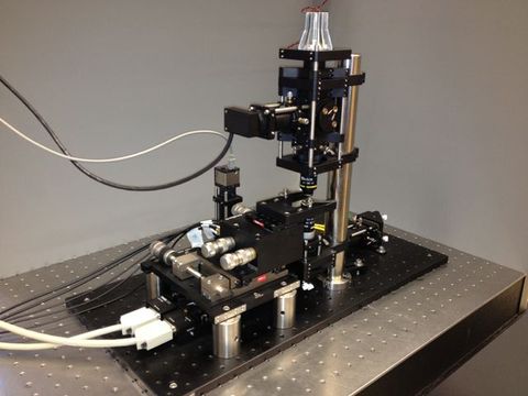
| − | | [[Image:OpticalTrap.JPG|thumb|center|top|480px|Laser tweezers | + | | [[Image:OpticalTrap.JPG|thumb|center|top|480px|Laser tweezers constructed from optical components in the MIT Bioinstrumentation Teaching Lab. [http://www.thorlabs.com ThorLabs] offers a kit that includes the parts needed to construct a similar instrument, part number [http://www.thorlabs.com/NewGroupPage9_PF.cfm?ObjectGroup_ID=3959 OTKB].]] |
|} | |} | ||
==Introduction== | ==Introduction== | ||
| − | Optical tweezers can exert | + | Optical tweezers can exert and measure forces on micron-scale dielectric particles. This capability offers a unique and valuable tool for manipulating and measuring cell components at the single molecule level. For example, optical traps have been used extensively to investigate the mechanical properties of biological polymers and the force generation mechanisms of molecular motors. In many studies, optical tweezers apply force to functionalized microspheres, which act as convenient handles attached to molecules of interest. |
To make quantitative force measurements, the instrument records the displacement of a trapped microsphere over time. For small displacements, the exerted force is very nearly proportional to displacement, so the trap can be modeled as a linear spring. Accurate force and position measurements depend on careful calibration of the position detector responsivity, G, and the trap stiffness α, also called the spring constant. The stiffness is a function of trapping laser power, bead size, bead composition, and optical properties of the sample. | To make quantitative force measurements, the instrument records the displacement of a trapped microsphere over time. For small displacements, the exerted force is very nearly proportional to displacement, so the trap can be modeled as a linear spring. Accurate force and position measurements depend on careful calibration of the position detector responsivity, G, and the trap stiffness α, also called the spring constant. The stiffness is a function of trapping laser power, bead size, bead composition, and optical properties of the sample. | ||
| Line 13: | Line 13: | ||
==Instrument overview== | ==Instrument overview== | ||
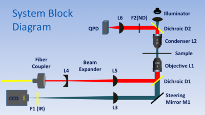
| − | + | [[Image:OpticalTrapBlockDiagram.PNG|thumb|right|400px|'''Optical trap block diagram.''']] | |
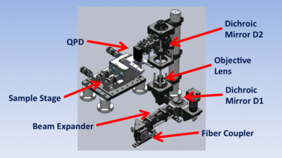
| − | [[Image:OpticalTrapBlockDiagram.PNG|thumb|right|400px|Optical trap block diagram.]] | + | [[Image:OpticalTrapLayout.PNG|thumb|right|400px|'''Optical trap layout.''' This diagram shows the locations of key optical trap components.]] |
| − | + | The trap is built around a 1.25NA, 100x, oil-immersion microscope objective lens (L1). The objective performs the dual functions of imaging the sample and focusing the trapping laser. The illumination source is an ultra-bright, blue LED. L7 focuses light from the LED on the back aperture of condenser lens L2 to produce collimated illumination. (L2 is a 10X, 0.25 NA microscope objective.) Tube lens L3 forms an image of the sample on a CCD camera. IR blocking filter F1 prevents the powerful trapping beam from damaging the camera. Steering mirror M1 allows adjustment of the field of view. | |
| − | + | The 975 nm, fiber-coupled trapping laser has a peak power output of 330 mW. A [http://www.thorlabs.com/newgrouppage9.cfm?objectgroup_id=2940 fiber coupler] produces a collimated beam in free space. The fiber coupler is followed by a Galilean telescope (lenses L4 and L5) that expands the beam by a factor of four in order to fill the back aperture of L1. Dichroic mirror D1 redirects the expanded beam toward the objective lens. L1 brings the beam to a sharp focus, which forms the trap. | |
| − | + | A quadrant photodiode (QPD) generates voltages used for detecting position of a trapped particle. Laser light that passes through the sample is collected by condenser L2 and diverted toward the QPD by dichroic mirror D2. To facilitate detection, L6 focuses the back aperture of the condenser (L2) on to the QPD. Neutral density filter F2 reduces the intensity of the beam to prevent damage to the QPD. | |
| − | + | A three axis stage with a combination of micrometer and closed-loop piezo drives positions the sample above the objective. The piezos have a range of about twenty microns. | |
| − | + | The optical trap in the demonstration was developed in the MIT Bioinstrumentation Teaching Lab. Thorlabs offers a [kit that includes all of the bits needed to make the trap, [http://www.thorlabs.com/NewGroupPage9_PF.cfm?ObjectGroup_ID=3959 part number OTKB]. | |
| − | [[ | + | |
| − | == | + | Setup and alignment of the instrument is detailed on [http://measure.mit.edu/~20.309/wiki/index.php?title=Aligning_the_optical_trap this page]. |
| + | |||
| + | ==Calibration== | ||
| + | For small displacements, the optical force is very nearly proportional to displacement. In this range, the trap can be modeled as a linear spring that follows Hooke's law: <i>F = -α x</i>. The QPD position detector produces a voltage signal. For small displacements, the voltage varies in proportion to the distance from the trap center to the particle according to the relation <i>x = G<sub>QPD</sub> V</i>.To make quantitative force measurements, both <i>G<sub>QPD</sub></i> and <i>α</i> must be known. | ||
| + | |||
| + | Accurate force and position measurements depend on careful calibration of G<sub>QPD</sub> and α. G<sub>QPD</sub> and α are functions of the adjustment of the instrument, trapping laser power, bead size, bead composition, and optical properties of the sample. The instrument has to be calibrated for each type of sample and any time an adjustment is made. (Calibration can be sensitive to the angle of the sample chamber, so it is a good idea to recalibrate every time the sample is changed.) | ||
| + | |||
| + | ===Finding α=== | ||
| + | Several methods for measuring trap stiffness have been developed. Because the methods rely on different underlying principles, they tend to be sensitive to different types of experimental errors. Using multiple calibration methods can provide an important check on results. | ||
| + | |||
| + | ====Equipartition method==== | ||
| + | The first method for estimating the trap stiffness α takes relies on the thermal excitation of a trapped particle by collissions with solvent molecules. The equipartitoin theorem asserts that the average potential energy of a trapped particle equals the average thermal energy of solvent molecules it is suspended in: ½ k<sub>B</sub> θ = 〈½ αx<sup>2</sup>〉, where k<sub>B</sub> is Boltzmann’s constant, θ is the temperature, x is a vector of displacement samples, and 〈 〉 is the expected value operator. | ||
| + | |||
| + | To calculate the stiffness by this method, convert QPD voltages for a sample of X- and Y- positions to distance units using GQPD. Take the variance of the X- and Y-position signals and solve for α. | ||
| + | |||
| + | ====PSD method==== | ||
| + | |||
| + | ====Stokes method==== | ||
| + | |||
| + | ====Summary==== | ||
| + | |||
| + | The following table summarizes the three methods: | ||
<table class="wikitable" style="text-align:center"> | <table class="wikitable" style="text-align:center"> | ||
| − | <caption style="font-size: | + | <caption style="font-size:14pt">Trap stiffness calibration methods and sensitivity to measurement parameters</caption> |
<tr> | <tr> | ||
<th scope="col" rowspan="2">Method</th> | <th scope="col" rowspan="2">Method</th> | ||
| Line 52: | Line 72: | ||
<tr> | <tr> | ||
<th scope="row">Equipartition</th> | <th scope="row">Equipartition</th> | ||
| − | <td><math>\frac{K_B T}{\langle R_{ | + | <td><math>\frac{K_B T}{\langle R_{qpd} V_{qpd} \rangle ^ 2}</math></td> |
<td>inverse square</td> | <td>inverse square</td> | ||
<td>none</td> | <td>none</td> | ||
| Line 74: | Line 94: | ||
<tr> | <tr> | ||
<th scope="row">Stokes</th> | <th scope="row">Stokes</th> | ||
| − | <td><math>\langle \frac{3 \pi \eta d \, R_{stage} \, ^{d V_{stage}} / _{dt}} { | + | <td><math>\langle \frac{3 \pi \eta d \, R_{stage} \, ^{d V_{stage}} / _{dt}} {R_{qpd} V_{qpd}} \rangle</math></td> |
<td>inverse</td> | <td>inverse</td> | ||
<td>linear</td> | <td>linear</td> | ||
| Line 85: | Line 105: | ||
</table> | </table> | ||
| − | == | + | ===Finding G<sub>QPD</sub>=== |
| − | + | Similarly, there are several ways to measure G<sub>QPD</sub> — each with its own strengths and weaknesses. | |
| − | + | ||
| − | + | ||
| − | + | ||
| − | + | ||
| − | + | ||
| − | + | ||
| − | < | + | |
| − | < | + | |
| − | + | ||
| − | + | ||
| − | + | ||
| − | < | + | |
| − | < | + | |
| + | ==Making a calibration sample== | ||
| + | |||
| + | <html> | ||
| + | <div align="center"> | ||
| + | <table border="1"> | ||
| + | <tr><td> | ||
| + | <iframe src="http://techtv.mit.edu/embeds/23503?size=custom&custom_width=544&player=simple&external_stylesheet=" frameborder="0" width="544" height="338"></iframe> | ||
| + | </td></tr> | ||
| + | <tr><td> | ||
| + | <b><div align="center">Making a calibration sample</div></b> | ||
| + | </td></tr> | ||
| + | </table> | ||
| + | </div> | ||
</html> | </html> | ||
| + | |||
| + | |||
==OTKB software== | ==OTKB software== | ||
| Line 107: | Line 129: | ||
<html> | <html> | ||
| − | < | + | <div align="center"> |
| − | < | + | <table border="1"> |
| − | + | <tr><td> | |
| − | + | <iframe src="http://techtv.mit.edu/embeds/_203822?size=custom&custom_width=544&player=simple&external_stylesheet=" frameborder="0" width="544" height="338"></iframe> | |
| − | + | </td></tr> | |
| − | + | <tr><td> | |
| + | <b><div align="center">Starting the software</div></b> | ||
| + | </td></tr> | ||
| + | </table> | ||
| + | </div> | ||
</html> | </html> | ||
| Line 122: | Line 148: | ||
===Stokes method=== | ===Stokes method=== | ||
<html> | <html> | ||
| − | < | + | <div align="center"> |
| − | < | + | <table border="1"> |
| − | + | <tr><td> | |
| − | + | <iframe src="http://techtv.mit.edu/embeds/_203822?size=custom&custom_width=544&player=simple&external_stylesheet=" frameborder="0" width="544" height="338"></iframe> | |
| − | + | </td></tr> | |
| − | + | <tr><td> | |
| + | <b><div align="center">Starting the software</div></b> | ||
| + | </td></tr> | ||
| + | </table> | ||
| + | </div> | ||
</html> | </html> | ||
| + | |||
{{Template:20.309 bottom}} | {{Template:20.309 bottom}} | ||
Latest revision as of 12:53, 7 May 2013
Introduction
Optical tweezers can exert and measure forces on micron-scale dielectric particles. This capability offers a unique and valuable tool for manipulating and measuring cell components at the single molecule level. For example, optical traps have been used extensively to investigate the mechanical properties of biological polymers and the force generation mechanisms of molecular motors. In many studies, optical tweezers apply force to functionalized microspheres, which act as convenient handles attached to molecules of interest.
To make quantitative force measurements, the instrument records the displacement of a trapped microsphere over time. For small displacements, the exerted force is very nearly proportional to displacement, so the trap can be modeled as a linear spring. Accurate force and position measurements depend on careful calibration of the position detector responsivity, G, and the trap stiffness α, also called the spring constant. The stiffness is a function of trapping laser power, bead size, bead composition, and optical properties of the sample.
This page has tips for setting up and aligning an optical trap. It discusses three methods for obtaining the spring constant and two methods for measuring α.
Instrument overview
The trap is built around a 1.25NA, 100x, oil-immersion microscope objective lens (L1). The objective performs the dual functions of imaging the sample and focusing the trapping laser. The illumination source is an ultra-bright, blue LED. L7 focuses light from the LED on the back aperture of condenser lens L2 to produce collimated illumination. (L2 is a 10X, 0.25 NA microscope objective.) Tube lens L3 forms an image of the sample on a CCD camera. IR blocking filter F1 prevents the powerful trapping beam from damaging the camera. Steering mirror M1 allows adjustment of the field of view.
The 975 nm, fiber-coupled trapping laser has a peak power output of 330 mW. A fiber coupler produces a collimated beam in free space. The fiber coupler is followed by a Galilean telescope (lenses L4 and L5) that expands the beam by a factor of four in order to fill the back aperture of L1. Dichroic mirror D1 redirects the expanded beam toward the objective lens. L1 brings the beam to a sharp focus, which forms the trap.
A quadrant photodiode (QPD) generates voltages used for detecting position of a trapped particle. Laser light that passes through the sample is collected by condenser L2 and diverted toward the QPD by dichroic mirror D2. To facilitate detection, L6 focuses the back aperture of the condenser (L2) on to the QPD. Neutral density filter F2 reduces the intensity of the beam to prevent damage to the QPD.
A three axis stage with a combination of micrometer and closed-loop piezo drives positions the sample above the objective. The piezos have a range of about twenty microns.
The optical trap in the demonstration was developed in the MIT Bioinstrumentation Teaching Lab. Thorlabs offers a [kit that includes all of the bits needed to make the trap, part number OTKB.
Setup and alignment of the instrument is detailed on this page.
Calibration
For small displacements, the optical force is very nearly proportional to displacement. In this range, the trap can be modeled as a linear spring that follows Hooke's law: F = -α x. The QPD position detector produces a voltage signal. For small displacements, the voltage varies in proportion to the distance from the trap center to the particle according to the relation x = GQPD V.To make quantitative force measurements, both GQPD and α must be known.
Accurate force and position measurements depend on careful calibration of GQPD and α. GQPD and α are functions of the adjustment of the instrument, trapping laser power, bead size, bead composition, and optical properties of the sample. The instrument has to be calibrated for each type of sample and any time an adjustment is made. (Calibration can be sensitive to the angle of the sample chamber, so it is a good idea to recalibrate every time the sample is changed.)
Finding α
Several methods for measuring trap stiffness have been developed. Because the methods rely on different underlying principles, they tend to be sensitive to different types of experimental errors. Using multiple calibration methods can provide an important check on results.
Equipartition method
The first method for estimating the trap stiffness α takes relies on the thermal excitation of a trapped particle by collissions with solvent molecules. The equipartitoin theorem asserts that the average potential energy of a trapped particle equals the average thermal energy of solvent molecules it is suspended in: ½ kB θ = 〈½ αx2〉, where kB is Boltzmann’s constant, θ is the temperature, x is a vector of displacement samples, and 〈 〉 is the expected value operator.
To calculate the stiffness by this method, convert QPD voltages for a sample of X- and Y- positions to distance units using GQPD. Take the variance of the X- and Y-position signals and solve for α.
PSD method
Stokes method
Summary
The following table summarizes the three methods:
| Method | Equation | QPD Responsivity | Stage Responsivity | Solvent Viscosity | Particle Diameter | Temperature | Technical Noise |
|---|---|---|---|---|---|---|---|
| $ R_{QPD} $ | $ R_{stage} $ | $ \eta $ | $ d $ | $ T $ | |||
| Equipartition | $ \frac{K_B T}{\langle R_{qpd} V_{qpd} \rangle ^ 2} $ | inverse square | none | none | none | linear and indirect (viscosity change) | systematic decrease |
| PSD | $ \left. {6 \pi^2 \eta d \, f_0} \right. $ | none | none | linear | linear | indirect (viscosity change) | small |
| Stokes | $ \langle \frac{3 \pi \eta d \, R_{stage} \, ^{d V_{stage}} / _{dt}} {R_{qpd} V_{qpd}} \rangle $ | inverse | linear | linear | linear | indirect (viscosity change) | none |
Finding GQPD
Similarly, there are several ways to measure GQPD — each with its own strengths and weaknesses.
Making a calibration sample
<html>
|
<iframe src="http://techtv.mit.edu/embeds/23503?size=custom&custom_width=544&player=simple&external_stylesheet=" frameborder="0" width="544" height="338"></iframe> |
|
Making a calibration sample
|
</html>
OTKB software
Starting the software
<html>
|
<iframe src="http://techtv.mit.edu/embeds/_203822?size=custom&custom_width=544&player=simple&external_stylesheet=" frameborder="0" width="544" height="338"></iframe> |
|
Starting the software
|
</html>
Calibration
Measuring R by scanning a stuck bead
PSD method
Equipartition method
Stokes method
<html>
|
<iframe src="http://techtv.mit.edu/embeds/_203822?size=custom&custom_width=544&player=simple&external_stylesheet=" frameborder="0" width="544" height="338"></iframe> |
|
Starting the software
|
</html>


