Difference between revisions of "DNA Melting: Simulating DNA Melting - Basics"
(→Modeling dsDNA equilibrium concentraion) |
(→Modeling dsDNA equilibrium concentraion) |
||
| Line 40: | Line 40: | ||
* Plotting data | * Plotting data | ||
| − | ==Modeling dsDNA equilibrium | + | ==Modeling dsDNA equilibrium fraction== |
| − | We derived an expression for dsDNA | + | We derived an expression for dsDNA fraction at a given temperature [[DNA Melting Thermodynamics#Simulating DNA Melting|in class]]: |
:<math> | :<math> | ||
K_{eq} = e^\left [\frac{\Delta S^{\circ}}{R} - \frac{\Delta H^{\circ}}{R T} \right ] | K_{eq} = e^\left [\frac{\Delta S^{\circ}}{R} - \frac{\Delta H^{\circ}}{R T} \right ] | ||
| Line 48: | Line 48: | ||
f = \frac{1 + C_T K_{eq} - \sqrt{1 + 2 C_T K_{eq}}}{C_T K_{eq}} | f = \frac{1 + C_T K_{eq} - \sqrt{1 + 2 C_T K_{eq}}}{C_T K_{eq}} | ||
</math> | </math> | ||
| + | |||
| + | where ''C_T'' is the total concentration of DNA strands. | ||
Since this is a complicated equation that we will evaluate many times, it makes sense to write a Matlab function. | Since this is a complicated equation that we will evaluate many times, it makes sense to write a Matlab function. | ||
===dsDNA fraction function=== | ===dsDNA fraction function=== | ||
| − | The fraction of dsDNA is a function of 4 variables: ''ΔS°'', ''ΔH°'', temperature, and concentration. The <tt>DnaFraction</tt> function below also takes an optional fifth argument for the gas constant | + | The fraction of dsDNA is a function of 4 variables: ''ΔS°'', ''ΔH°'', temperature, and concentration. The <tt>DnaFraction</tt> function below also takes an optional fifth argument for the gas constant to enable using different unit systems. Using the element-by-element divide operator in the body of the function makes it possible for <tt>DnaFraction</tt> to accept either a single temperature argument or a vector of temperature values. (As a general rule, use the <tt>./</tt> operator instead of <tt>/</tt> unless you intend to do a matrix divide.) |
The Matlab function <tt>nargin</tt> returns the number of arguments that the function was called with. Many Matlab programs use this function to handle variable numbers of arguments. If <tt>nargin</tt> returns 4 or less, <tt>R</tt> is set to the default value of 1.987. Otherwise, the value of <tt>R</tt> is set to the value supplied by the caller. | The Matlab function <tt>nargin</tt> returns the number of arguments that the function was called with. Many Matlab programs use this function to handle variable numbers of arguments. If <tt>nargin</tt> returns 4 or less, <tt>R</tt> is set to the default value of 1.987. Otherwise, the value of <tt>R</tt> is set to the value supplied by the caller. | ||
| Line 103: | Line 105: | ||
ideal.deltaS = -184; % cal/mol | ideal.deltaS = -184; % cal/mol | ||
ideal.deltaH = -71E3; % cal/(mol K) | ideal.deltaH = -71E3; % cal/(mol K) | ||
| − | ideal.DnaConcentration = 30E-6; | + | ideal.DnaConcentration = 30E-6; % &M |
% call DnaFraction function | % call DnaFraction function | ||
| Line 131: | Line 133: | ||
:<math> | :<math> | ||
{f'}_N = \frac{f_{N+1}-f_{N}}{\Delta T}</math>. | {f'}_N = \frac{f_{N+1}-f_{N}}{\Delta T}</math>. | ||
| − | '' | + | ''df/dT'' is guaranteed to take on the value given by ''f'<sub>N</sub>'' at some point between ''NΔT'' and ''(N+1)ΔT''; however, this happy coincidence can occur at any place in the interval. A simple but effective technique is to guess that equality occurs in the middle of the interval. This guess is close enough in most cases. |
The code below computes the finite difference and stores it in the <tt>dDsDnaFraction</tt> field of <tt>ideal</tt>. It also generates an associated temperature vector (<tt>ideal.dTemperature</tt>) with values centered between the original temperature samples. Note that both vectors are one element shorter than the original data. | The code below computes the finite difference and stores it in the <tt>dDsDnaFraction</tt> field of <tt>ideal</tt>. It also generates an associated temperature vector (<tt>ideal.dTemperature</tt>) with values centered between the original temperature samples. Note that both vectors are one element shorter than the original data. | ||
| Line 137: | Line 139: | ||
<pre> | <pre> | ||
ideal.dTemperature = ideal.temperature(1:99) + 0.5; % create new temperature vector | ideal.dTemperature = ideal.temperature(1:99) + 0.5; % create new temperature vector | ||
| − | ideal.dDsDnaFraction = diff(ideal.dsDnaFraction); % take the difference | + | ideal.dDsDnaFraction = diff(ideal.dsDnaFraction); % take the difference between adjacent elements of the DnaFraction series |
figure(2) | figure(2) | ||
Revision as of 14:39, 17 August 2012
Introduction
Chance favors the prepared mind.
—Louis Pasteur (abridged)
This tutorial will show you how to simulate the DNA melting experiment with Matlab. The DNA melting apparatus you will build produces two output voltages related to the sample temperature and fluorescence intensity. During an experimental run, these two voltages will be recorded periodically. At the end of this tutorial, you will be able to produce mock datasets that are similar to what you will record in the lab. You can use simulated datasets to help develop and debug your data analysis scripts.
It is essential to have working data analysis scripts before you begin running experiments in the lab.
The procedure for creating the simulation is:
- Write a function to compute the equilibrium dsDNA concentration vs. temperature
- Model sample temperature versus time during an experimental run
- Compute the RTD voltage from temperature vs. time data
- Compute relative fluorescence intensity vs. time data from temperature vs. time data
Run Matlab and follow along as you read. Code from this page can be copied and pasted into the Matlab command window.
If you prefer to work in Python, please see this page.
Before you begin
- Review the DNA Melting Thermodynamics Notes.
- If you need a review of Matlab fundamentals, see Matlab Fundamentals tutorial.
Matlab skills
- Array arithmetic (element-by-element) operators (+, -, .*, ./)
- Functions declared in an m-file
- Conditionals
- Functions that take a variable number of arguments
- Numerical differentiation
- Plotting data
Modeling dsDNA equilibrium fraction
We derived an expression for dsDNA fraction at a given temperature in class:
- $ K_{eq} = e^\left [\frac{\Delta S^{\circ}}{R} - \frac{\Delta H^{\circ}}{R T} \right ] $
- $ f = \frac{1 + C_T K_{eq} - \sqrt{1 + 2 C_T K_{eq}}}{C_T K_{eq}} $
where C_T is the total concentration of DNA strands.
Since this is a complicated equation that we will evaluate many times, it makes sense to write a Matlab function.
dsDNA fraction function
The fraction of dsDNA is a function of 4 variables: ΔS°, ΔH°, temperature, and concentration. The DnaFraction function below also takes an optional fifth argument for the gas constant to enable using different unit systems. Using the element-by-element divide operator in the body of the function makes it possible for DnaFraction to accept either a single temperature argument or a vector of temperature values. (As a general rule, use the ./ operator instead of / unless you intend to do a matrix divide.)
The Matlab function nargin returns the number of arguments that the function was called with. Many Matlab programs use this function to handle variable numbers of arguments. If nargin returns 4 or less, R is set to the default value of 1.987. Otherwise, the value of R is set to the value supplied by the caller.
Matlab notes: Matlab functions must be saved in the current directory or another directory in the Matlab path. The name of the file must be the function name appended with ".m". Function help should be placed in comments at the top of the file. Type help DnaFraction to see how this works.
% Returns the fraction of dsDNA in a solution containing equal concentrations
% of two complementary DNA oligos as a functino of total DNA concentration,
% temperature, entropy change, and enthalpy change.
% Gas constant is an optional parameter.
%
% USAGE: f = DnaFraction(Ct, T, DeltaS, DeltaH, <GasConstant>)
% RETURN VALUE: fraction of dsDNA
%
% Default units are molar, Kelvin, cal/mole, and cal/(mole-Kelvin). For
% other unit systems, supply the appropriate value of R in the optional
% fifth parameter. The default value is 1.987 cal/(degree K * mole).

function f = DnaFraction(Ct, T, DeltaS, DeltaH, GasConstant)
% Gas constant
if(nargin < 5)              % determine if caller supplied R value or not
    R = 1.987;              % set to default: cal/(degree K * mole)
else
    R = GasConstant;        % otherwise use caller's value
end

% Compute Ct * Keq
CtKeq = Ct * exp(DeltaS / R - DeltaH ./ (R * T));

%now compute f
f = (1 + CtKeq - sqrt(1 + 2 * CtKeq)) ./ CtKeq;

% Written 4/9/2008 by SCW
Plot an ideal melting curve
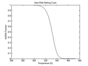
Does the DnaFraction function work as expected? A good way to test the function is to plot a melting curve generated by DnaFraction.
Matlab notes: Over the course of an interactive Matlab session, you may run several simulations with different parameters. Using a structure to keep the results of each simulation together is a good way to prevent the workspace from becoming disorganized. The struct function creates an empty structure. In the code below, a structure called ideal is created to hold the ideal melting curve data. (Since variables are dynamically allocated and typed in Matlab, the struct command is optional; however, explicitly creating the structure can make your code easier to read and better performing.)
Since DnaFraction accepts a vector temperature argument, an entire melting curve can be computed with a single call.
close all;
clc;

ideal = struct();                          % create an empty structure to hold the results
ideal.temperature = (0:99) + 273.15;       % temperature axis in Kelvin: 100 points(0-99C)
ideal.deltaS = -184;                       % cal/mol
ideal.deltaH = -71E3;                      % cal/(mol K)
ideal.DnaConcentration = 30E-6;    % &M

% call DnaFraction function
% arguments: concentration, temperature vector, delta S, delta H
% (optional R argument not supplied)

ideal.dsDnaFraction = DnaFraction(ideal.DnaConcentration, ...
    ideal.temperature, ideal.deltaS, ideal.deltaH);

figure(1)
plot(ideal.temperature, ideal.dsDnaFraction);
title('Ideal DNA Melting Curve');
xlabel('Temperature (K)');
ylabel('dsDNA Fraction');
Experiment with different values of ΔS° and ΔH° to see how the curve changes.
Also several web tools are available to predict the melting temperature. See, for example, DINA Melt or Oligocalc. You can use one of these or another tool to estimate values for different DNA sequences.
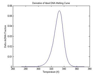
One method of estimating Tm is to find the temperature where the dsDNA fraction equals 1/2. Another method is to differentiate the melting curve. Tm occurs at the peak of the derivative — where the dsDNA fraction is changing the fastest. (Why might you prefer one method over the other when estimating Tm from experimental data?)
Numerical differentiation
The fluorescence function fN is a sampled version of the continuous function f(T) such that fN = f(NΔT), where ΔT is the sampling interval (1° C, in this instance). One method for computing a numerical approximation to df/dT is the finite difference:
- $ {f'}_N = \frac{f_{N+1}-f_{N}}{\Delta T} $.
df/dT is guaranteed to take on the value given by f'N at some point between NΔT and (N+1)ΔT; however, this happy coincidence can occur at any place in the interval. A simple but effective technique is to guess that equality occurs in the middle of the interval. This guess is close enough in most cases.
The code below computes the finite difference and stores it in the dDsDnaFraction field of ideal. It also generates an associated temperature vector (ideal.dTemperature) with values centered between the original temperature samples. Note that both vectors are one element shorter than the original data.
ideal.dTemperature = ideal.temperature(1:99) + 0.5; % create new temperature vector
ideal.dDsDnaFraction = diff(ideal.dsDnaFraction);   % take the difference between adjacent elements of the DnaFraction series

figure(2)
plot(ideal.dTemperature, -1 * ideal.dDsDnaFraction);
title('Derivative of Ideal DNA Melting Curve');
xlabel('Temperature (K)');
ylabel('Delta dsDNA Fraction');
In the previous section, the plot shows that the dsDNA fraction equals 0.5 at about 332.5 degrees. The peak of the derivative also occurs at the same temperature. (The curve is plotted inverted.)
Set up simulation conditions and data structure
It will be convenient to set up a data structure with the simulation parameters and a time axis.
sim1 = struct();                                          % create empty struct for sim results
sim1.DnaConcentration = 30E-6;                            % 30 micromolar concentration
sim1.deltaS = ideal.deltaS;                               % cal / (mole-K)
sim1.deltaH = ideal.deltaH;                               % cal / mole
sim1.finalTemperature = 293;                              % approx. room temperature
sim1.sampleRate = 1;                                      % 1 Hz sample rate
sim1.durationHT = 900;                                    % heating time, s
sim1.durationCL = 600;                                    % cooling time, s
sim1.timeHT = (0:(1/sim1.sampleRate):sim1.durationHT)';   % heating time vector, s
sim1.timeCL = (2:(1/sim1.sampleRate):sim1.durationCL)';   % cooling time vector, s
sim1.time = [sim1.timeHT; sim1.timeHT(end)+sim1.timeCL];  % complete time vector, s
Simulate sample temperature during an experimental run
The goal of the simulation is to produce two simulated voltage signals that resemble what you will measure in the lab. Since both of the voltages are functions of temperature, it makes sense to begin by modeling how the sample temperature behaves during an experimental run.
Sample heating and cooling
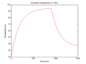
During each experimental run, the range of temperatures will be provided by forced heating by a TEC, followed by natural cooling of the sample after the heat source is switched off. At the beginning of an experimental run the sample will be at room temperature, then the TEC is switched on and the DNA + fluorescent dye sample is heated to 95°C in about 5 minutes. Upon reaching 95°C, the TEC power is switched off. Then over a period of about 15 minutes, the sample cools to room temperature (less than 30°C). The rate of cooling is proportional to the difference between the sample's temperature and the room temperature, so the sample cools more quickly at the start of the experiment than near the end. (It can be frustrating to wait for the final few degrees.)
Both heating and cooling can be approximated by an exponential function. Heating is modeled with a time constant of about 1 minute, while cooling is modeled with a time constant of about 3 minutes. The equation for temperature (in K) versus time is:
- $ T_{heating}(t) = (T_{max} - T_i) (1 - e ^ {-\frac{t_{HT}}{\tau_{HT}}}) + T_i $
- $ T_{cooling}(t) = (T_{max} - T_f) e ^ {-\frac{t_{CL}}{\tau_{CL}}} + T_f $
where,
- T(t) is the temperature as a function of time,
- Ti is the initial temperature, likely room temperature,
- Tmax is the max temperature reached during the heating phase,
- Tf is the final temperature, likely not quite room temperature,
- τ is the time constant for heating (HT) and cooling (CL).
In Matlab:
sim1.heatingConstant = 180;                               % heating rate constant, 1/s
sim1.coolingConstant = 180;                               % cooling rate constant, 1/s
sim1.maxTemperature = 95 + 273;                           % target maximum sample temp, K
sim1.initialTemperature = 20 + 273;                       % starting room temp, K
sim1.finalTemperature = 35 + 273;                         % final cool-down temp, K

% use exp function to model exponential heating and cooling
sim1.temperature = ...
    [ (sim1.maxTemperature - sim1.initialTemperature)   ... % (T_max - T_i) *
    .* (1 - exp(-sim1.timeHT ./ sim1.heatingConstant))  ... % (1 + e^(-t/tauHT)) +
    + sim1.initialTemperature; ...                          % T_i
    (sim1.maxTemperature - sim1.finalTemperature)   ...     % (T_max - T_f) *
    .* exp(-sim1.timeCL ./ sim1.coolingConstant)  ...       % e^(-t/tauCL) +
    + sim1.finalTemperature ];                              % T_f

figure(3)
plot(sim1.time, sim1.temperature-273, 'r');
xlabel('Time (sec)');
ylabel('Temperature (C)');
title('Simulated Temperature vs. Time');
If you have any questions about the element-by-element division operator in Matlab (./), or the use of a semicolon for concatenation, see:this page or ask an Instructor or TA.
RTD temperature sensor model
RTD and voltage divider circuit
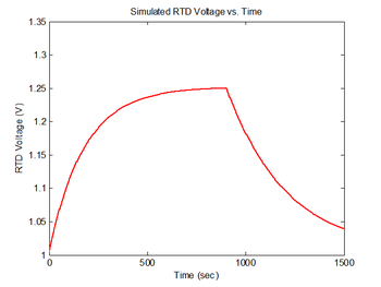
The resistance of the RTD is given by the equation $ R_{RTD} = R_o*(1 + \alpha \Delta T) $, where "α" is the temperature coefficient of resistance (TCR) for the RTD and $ R_o $ is the resistance at the reference temperature for the RTD. In the experimental apparatus, the RTD is hooked up as one element of a voltage divider with a pull-up resistor, R. The power supply input is 15 volts. Thus, the output voltage is: $ V_{RTD} = 15 * R_{RTD}/(R + R_{RTD}) $. The following code calculates RTD voltage measurements from sim1.temperature and stores the result in sim1.V_RTD, assuming $ R $ = 15kΩ, $ R_o $ = 1000Ω, $ \alpha $ = 3850 ppm/°C, and $ \Delta T $ is the difference, in Kelvin or Celsius, between the RTD reference temperature and the RTD temperature.
sim1.R_RTD_atZeroC = 1000;                                % Datasheet value of reference RTD resistance, C
sim1.RTDalpha = 3850;                                     % Datasheet value of RTD TCR, ppm/C
sim1.R_RTD = sim1.R_RTD_atZeroC ...
    * (1 + sim1.RTDalpha*1e-6 * (sim1.temperature-273));  % Compute RTD resistance, Ohms
sim1.R_pullup = 15e3;                                     % Pull-up resistor in voltage divider, Ohms
sim1.V_input = 15;                                        % Input voltage of divider, V
sim1.V_RTD = sim1.V_input * sim1.R_RTD ...
    ./ (sim1.R_pullup + sim1.R_RTD);                      % RTD votlage drop, V

figure(4)
plot(sim1.time, sim1.V_RTD, 'r');
xlabel('Time (sec)');
ylabel('RTD Voltage (V)');
title('Simulated RTD Voltage vs. Time');
Simulate DNA fraction for this temperature profile
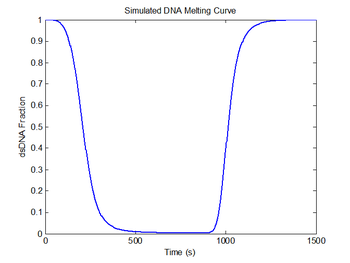
Use the DnaFraction function given above to calculate the simulated fluorescence using the combined heating and cooling temperature profile that you just calculated.
sim1.dsDnaFraction = DnaFraction(sim1.DnaConcentration, ...
    sim1.temperature, sim1.deltaS, sim1.deltaH);

figure(5)
plot(sim1.time, sim1.dsDnaFraction);
title('Simulated DNA Melting Curve');
xlabel('Time (s)');
ylabel('dsDNA Fraction');

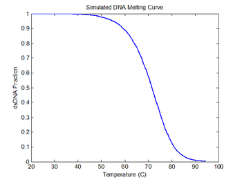
figure(6)
plot(sim1.temperature-273, sim1.dsDnaFraction);
title('Simulated DNA Melting Curve');
xlabel('Temperature (C)');
ylabel('dsDNA Fraction');
Analyze simulated data
Fitting the model
To perform the fit, use the matlab function from above, DnaFraction. You can use ay of Matlab's least sqaures curve fitters to estimate best-fit values for ΔH° and ΔS°. We prefer (nlinfit) because it allows you to calculate confidence intervals.
nlinfit requires the fitting function to be implemented a particular way. You may find the following code excerpt, which declares a suitable function called myFunction, useful.
% Create user function for fitting
myFunction = @ (x, xdata)  DnaFraction(sim1.DnaConcentration, xdata, ...
    x(1), x(2));

% Fit data to model
fitOptions = optimset('TolFun',1E-30,'TolX',1E-10,'MaxFunEvals',1E4,...
    'MaxIter',1E4);
data = [sim1.temperature, sim1.dsDnaFraction];
[fitValues, residual, j, COVB, mse] = nlinfit(sim1.temperature, ...
    sim1.dsDnaFraction, myFunction, [sim1.deltaS, sim1.deltaH], fitOptions);
ParameterConfidenceInterval = nlparci(fitValues, residual, 'covar',...
    COVB);

sim1.fitDnaFraction = DnaFraction(sim1.DnaConcentration, ...
    sim1.temperature, fitValues(1), fitValues(2));

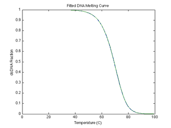
figure(7)
plot(sim1.temperature-273, sim1.dsDnaFraction, ...
    ideal.temperature-273, ideal.dsDnaFraction);
title('Fitted DNA Melting Curve');
xlabel('Temperature (C)');
ylabel('dsDNA Fraction');
At first glance there appears to be only one curve. This is what we expect for simulated data with no noise or other non-idealities. Close inspection of your plotted curves will show that there are distinct simulated data and fitted curves. The more interesting case is to add some simulated noise, bleaching, fluorescence variation with temperature, temperature lag, reaction rates, etc. Some of these will be covered in Intermediate Topics, and you can add any that are not covered there. Others will need to be included by you when you analyze your data.
Plot legends in Matlab
You can create fancier plots with a variety of lines colors and styles and legends. Annoyingly, Matlab handles legends differently than other plot commands. The hold command does not apply to the legend command. (Direct complaints to http://www.mathworks.com/support.) However, the following code excerpt is a work-around and adds a plot legend. This code runs after a main loop which would cycle the above fit routine through your multiple data sets (more on that later). In such an implementation, the cellular array out contains the results from processing. The code below also places an "X" at the melting temperature.
% Compute text cell array for plot legends and plot an
% "X" at the estimated melting temperature

for ii=1:length(out)
    legendText{2 * ii - 1} = sampleInfo{ii}.SampleName;
    legendText{2 * ii} = [sampleInfo{ii}.SampleName ' Best Fit'];
    figure(1)
    plot(out{ii}.maxDerivativeTemperature, out{ii}.fluorescence(out{ii}.maxDerivativeIndex),...
        'linewidth',2,'marker','x','markersize',18,'color',out{ii}.plotColor);
    plot(out{ii}.maxModelDerivativeTemperature, out{ii}.fitFluorescence(...
        out{ii}.maxModelDerivativeIndex), 'linewidth',2,'marker','x','markersize',18,'color',...
        out{ii}.modelPlotColor);
    figure(2)
    plot(out{ii}.maxDerivativeTemperature, out{ii}.dFdT(out{ii}.maxDerivativeIndex),...
        'linewidth',2,'marker','x','markersize',18,'color',out{ii}.plotColor);
    plot(out{ii}.maxModelDerivativeTemperature, out{ii}.dModelFdT(...
        out{ii}.maxModelDerivativeIndex), 'linewidth',2,'marker','x','markersize',18,'color',...
        out{ii}.modelPlotColor);
end

% Add the legends
figure
legend(legendText, 'location', 'southwest');
hold off;
figure
legend(legendText, 'location', 'southwest');
hold off;
Next Steps
After completing this tutorial, you are ready to move on to the Intermediate topics, adding noise and bleaching. With those wrinkles, it will be instructive for you to again try fitting a model to simulated data and discover how much the noise and bleaching affect your ability to estimate the true DNA melting curve. Then you will be ready to include the most significant in-practice difficulty we face with this lab: the temperature lag between the temperature measured at the heating block, and the actual temperature in the DNA sample.
Lab manual sections
- DNA Melting: Simulating DNA Melting - Basics
- DNA Melting Part 1: Measuring Temperature and Fluorescence
- DNA Melting Report Requirements for Part 1
- DNA Melting: Simulating DNA Melting - Intermediate Topics
- DNA Melting Part 2: Lock-in Amplifier and Temperature Control
- DNA Melting Report Requirements for Part 2

