Difference between revisions of "DNA Melting: Model function and parameter estimation by nonlinear regression"
(→Assumptions) |
(→Sample temperature) |
||
| Line 45: | Line 45: | ||
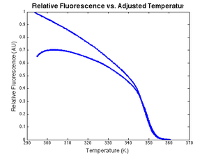
|[[Image:DNA melting data corrected for temperature lag.png|thumb|300px|right|<math>V_f</math> versus model sample temperature, <math>\theta_{sample}</math>.]] | |[[Image:DNA melting data corrected for temperature lag.png|thumb|300px|right|<math>V_f</math> versus model sample temperature, <math>\theta_{sample}</math>.]] | ||
|} | |} | ||
| + | |||
| + | ===Implementation=== | ||
| + | The Matlab functions{http://www.mathworks.com/help/control/ref/tf.html tf] and [http://www.mathworks.com/help/control/ref/lsim.html lsim] can be used to simulate this continuous-time system. Be certain to handle the initial conditions properly. (One way to avoid setting initial conditions is to subtract the initial value from the temperature signal and add it back in after evaluating <code>lsim</code>. | ||
==Photobleaching== | ==Photobleaching== | ||
Revision as of 18:30, 18 November 2012
Contents |
Overview
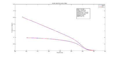
In addition to the dsDNA concentration, $ \Delta H^{\circ} $, and $ \Delta S^{\circ} $, the measured fluorescence voltage, $ V_{f,measured} $, depends of several factors, including:
- dynamics of the temperature cycling system
- thermal quenching of the fluorophore
- photobleaching
- responsivity and offset of the instrument
- binding kinetics of the dye
The goal is to write a model for $ V_f $ that takes these effects into account and use nonlinear regression to estimate the parameters.
Sample temperature
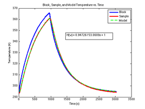
The DNA melter does not directly measure sample temperature. Sample temperature significantly lags block temperature.
Assumptions
- The RTD measures temperature of the metal heating block, which is uniform throughout.
- The heating block has a much larger heat capacity than the sample. (This allows the block to be modeled as a temperature source).
- The thermal capacity of the glass cuvette is small relative to its thermal resistance. (The cuvette's heat capacity is neglected in the model.)
- The sample has constant heat capacity and uniform temperature.
- Heat escapes from the sample to the environment at a rate proportional to the difference between the sample and room temperatures.
Under these assumptions, the thermal system can be modeled by lumped elements. An equivalent circuit for the heating system is shown in the figure. The circuit is a first-order, low-pass filter. In this circuit, a step increase in block temperature causes the sample temperature to rise exponentially to a peak value of $ K_{thermal} $ with time constant $ \tau_{thermal} $.
The transfer function of the low-pass filter has two parameters:
- $ K_{thermal} $ is the low frequency gain of the system.
- $ \tau $ is the time constant.
Implementation
The Matlab functions{http://www.mathworks.com/help/control/ref/tf.html tf] and lsim can be used to simulate this continuous-time system. Be certain to handle the initial conditions properly. (One way to avoid setting initial conditions is to subtract the initial value from the temperature signal and add it back in after evaluating lsim.
Photobleaching
Excited dye molecules can react chemically with compounds in their environment and permanently lose their ability to fluoresce — a phenomenon called photobleaching. LED and ambient light illuminate the SYBR Green dye for 15 or more minutes over the course of a single melting and annealing cycle, which results in measurable photobleaching. Bleaching can be diminished by lowering the illumination; however, the signal is also proportionally reduced. Photobleaching can also be corrected by a mathematical model.
Assumptions
Photobleaching is a complicated phenomenon. The model proposed here adheres to Dr. George E. P. Box's excellent advice on modeling. Some of the assumptions are more suspect than others.
Which assumptions are probably significant sources of systematic error?
- The dye is divided into two populations, bleached and unbleached, with concentrations S and S
- The initial dye concentration is S + S
- Only dye molecules bound to dsDNA may be excited.
- Only excited fluorophore molecules bleach
- An excited fluorophore will either bleach with probability $ p $ or return to the ground state with probability $ 1-p $.
- The constant $ 1-p $ encompasses all of the mechanisms by which the fluorophore returns to the ground state unbleached, including fluorescence, phosphorescence, and non-radiative relaxation.
- Bleaching is irreversible.
- The number of molecules in the excited state is proportional to fluorescence.
- Bleached and unbleached molecules bind to dsDNA with the same affinity.
Model
Under these assumptions, the bleaching rate is proportional to fluorescence.
$ K_{bleaching} $ encompasses several constants, including $ p $, illumination intensity, optical gain of the instrument, and lock-in amplifier gain.
Setting the initial dye concentration to 1, the fraction of unbleached SYBR Green can be calculated by integrating:
Background fluorescence (optional)
SYBR Green has a finite contrast ratio. In reality, unbound dye fluoresces at a low level. Because the model includes an arbitrary constant to account for instrument offset, the background fluorescence is not measured. Adding a constant rate term to the bleaching equation can help describe this behavior. The revised model is:
Many melting curves are well described without the constant term. If this term is not needed in your model, leave it out. A model that explains the dataset well with fewer parameters is always better.
Thermal quenching
SYBR Green I fluoresces less efficiently at higher temperatures. The decrease in fluorescence is approximately linear. Defining the dye efficiency at the initial temperature to be 1, quenching can be modeled by:
Instrument gain and offset
There are several optical and electronic gain factors built into the DNA melter that determine the instrument responsively, $ \partial V_F / \partial [{dsDNA}] $. In addition, $ V_f $ may be offset from zero when the dsDNA concentration is zero.
- $ K_{gain} $accounts for the arbitrary scale of$ V_f $.
- $ K_{offset} $ is equal to the value of $ V_f $ when the dsDNA concentration is zero.
Expression for model $ V_f $
DnaFraction is the melting curve model from part 1 of the lab.
Finding double stranded DNA fraction from raw data
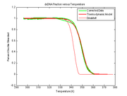
It is possible to use the inverse of the melting model function to transform raw experimental data into dsDNA fraction.
An example plot of $ \text{DnaFraction}(t)_{inverse-model} $ versus $ \theta_{sample} $ ishown at right. $ \text{DnaFraction}_{model} $ versus $ \theta_{sample} $is plotted on the same set of axes to reveals discrepancies between the model and experimental data caused by noise and systematic error in the model. These discrepancies are better visualized on a residual plot, as described below.
Residual plot
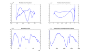
Observed values differ from predicted values because of noise and systematic errors in the model. Residuals are the difference between the experimental observations and the model predictions, $ V_{f,model}-V_{f,measured} $. Ideally, a plot of the residuals should demonstrate that the residuals are random and identically distributed — something like white noise.
The plots at right show $ V_{f,model}-V_{f,measured} $, plotted versus temperature, time, fluorescence, and the cumulative sum of fluorescence. The residuals are clearly not random and identically distributed. This suggests that the model does not perfectly explain the data. The scale of the plot is much smaller than the data plot — about one percent of the data scale.
The magnitude of the residuals is small, about one percent. A perfect model might require dozens of added parameters and additional physical measurements.
Plotting the residuals versus different variables can help suggest what factors are not modeled well.

