Converting Gaussian fit to Rayleigh resolution

Plot of an Airy function with Rayleigh resolution R=1, and a best-fit Gaussian function with σ=0.46869.

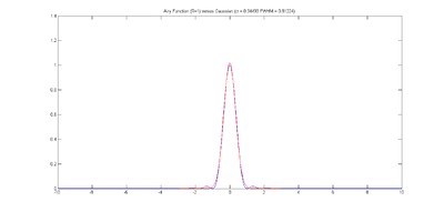
One method for measuring resolution is to fit a Gaussian function to an image of a very small source such as a fluorescent PSF microsphere. If the source is small enough, the image approximates the optical system's point spread function. As evidenced by the plot at right, the Gaussian function looks a lot like the central maximum of the Airy function.

The Rayleigh resolution of the Airy function shown is 1. The σ of the corresponding Gaussian is 0.46869. Thus, to convert the Gaussian fit to Rayliegh resolution, multiply σ by 1/0.46869 = 2.13361.

Note that a few Gaussian fitting functions (such as gaussfit) report sqrt(2) * σ. In this case, multiply σ by 1/(sqrt(2) * 0.46869) = 1.50869.

Here is the code that generated the plot:

xAxis = -10:0.01:10;

% generate an Airy disk profile with a normalized resolution R=1
firstBesselZero = 3.8317;
airyFunction = 2 * abs(besselj(1, firstBesselZero * xAxis)./ (firstBesselZero * xAxis));
airyFunction(xAxis == 0) = 1;

% use nonlinear regression to fit a Gaussian function to the Airy disk
gaussianFunction = @(parameters, xdata)  parameters(2) * exp( -xdata .^ 2 / (2 * parameters(1) .^ 2) );

bestFitGaussianParameters = nlinfit(xAxis, airyFunction, gaussianFunction, [1 1]);
lsqcurvefit(gaussianFunction, [1 1], xAxis, airyFunction);
bestFitGaussian = gaussianFunction(bestFitGaussianParameters, xAxis);
sigma = bestFitGaussianParameters(1);
sigmaToFwhmConversionFactor = 2 * sqrt(2*log(2));
fwhm = sigmaToFwhmConversionFactor * sigma;

% plot the results
plot(xAxis, airyFunction);
hold on;
plot(xAxis, bestFitGaussian, 'r');
title(texlabel(['Airy Function (R=1) versus Gaussian (sigma = ' num2str(sigma) ' FWHM = ' num2str(fwhm) ')']));