Assignment 9, Part 2: Simulating DNA melting data and testing the model function

This is Part 2 of Assignment 9.

Testing the fitting algorithm

Now it's time to test your code. Just like in the particle tracking assignment, we will create some simulated data with a known functional form, run the code, then see whether the outputs match what you put in.

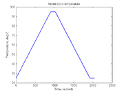
The input to the model function, V_f,model, is the block temperature (from which sample temperature is derived) and the model parameters (to be determined). In the next assignment, you will upgrade your DNA melting instrument to control the block temperature (rather than just having it turn on and off). You will produce a temperature ramp up from room temperature to 95 degrees, hold it there for a bit, then cool back down to room temperature. Let's simulate this in MATLAB:

Model block temperature.

% generate temperature ramp
Tmin = 25;
Tmax = 95;
Temp = [ (0:0.1:900)*((Tmax-Tmin)/900) + Tmin, Tmax*ones(1,1200), ...
    (0.1:0.1:900)*((Tmin-Tmax)/900) + Tmax, Tmin*ones(1,1200) ]';
time = (1:length(Temp))*0.1;
plot(time,Temp)
xlabel('Time, seconds')
ylabel('Temperature, deg C')
title('Model block temperature')

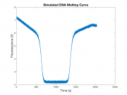
Next, create a synthetic data set to mimic the DNA fluorescence. We can start out simply, by omitting the effects of photobleaching and thermal quenching, but including the temperature delay between the block and sample.

dnaConcentration = 30E-6;
deltaS = -500;
deltaH = -180E3;
tauThermal = % choose some reasonable value
noise = 0.05;  % Roughly 5% noise

sampleTemp = SimulateLowPass(tauThermal, Temp);
F = DnaFraction( dnaConcentration, sampleTemp + 273, deltaS, deltaH );

Finally, and some random noise:

Noisy simulated DNA melting curve.

F = F + noise*randn(size(F));
plot(time,F)
xlabel('Temperature, deg C');
ylabel('Fluorescence Signal');
title('Simulated DNA Melting Curve');

Now that we have some synthetic data, we can test our fitting function and algorithm. The model function you wrote should be suitable for use with the Matlab nlinfit function (or other fitting routines). The input to nlinfit will then be the block temperature, fluorescence signal, the model function, and initial values of the model parameters. Additionally, there are many options you can set for the nlinfit algorithm [described here]. The output of nlinfit are the fitted parameter values.

fitValues = nlinfit(Temp, F, fitFunc, beta0, fitOptions);

The initial parameters you choose for nlinfit (beta0) are essential for getting a reasonable output. In this particular case, we know exactly what the parameters should be. Try altering the parameters slightly from their known values to get a feel for what it means for you guess to be 'reasonable'. Think about how you would guess the parameters for your future real data. Use these slightly altered parameters in the following plot.

a single plot showing: your simulated data your model function with initial best-guess parameters your model function with fitted parameters (obtained by nlinfit)

Even at a relatively large amplitude, random noise by itself should not appreciably affect the fitted parameter values; however, noise will generally contribute to uncertainty in the fit values. This uncertainty is seen in the parameter confidence intervals. Use the Matlab function nlparci to obtain the 95% confidence intervals from the results returned by nlinfit, e.g.,

    [fitValues, residual, ~, COVB, ~] = nlinfit(Temp, F, fitFunc, beta0, fitOptions);
    CI = nlparci(fitValues, residual, 'covar',COVB);

where CI will be an N×2 array of values where N is the length of fitValues.

a simulated DNA melting curve and vary the noise magnitude from 0 to 0.05. At each noise level, fit the curve, and compute the confidence intervals. Finally, plot the normalized confidence intervals as a function of the noise magnitude.