Difference between revisions of "20.109(S21):M1D7"
(→Introduction:Analyze ligand titration curves) |
(→Introduction:Analyze ligand titration curves) |
||
| Line 4: | Line 4: | ||
==Introduction:Analyze ligand titration curves == | ==Introduction:Analyze ligand titration curves == | ||
| − | Each protein in a cell collides with a tremendous variety of other molecules every second, but the great majority of these interactions are fleeting and have no functional consequences. However, in a small minority of these collisions, a more persistent interaction occurs between the protein and its ligand, docking the two into a precise relative orientation. This complex may stay assembled anywhere from seconds to days and perform a variety of functions: catalysis of a chemical reaction, construction of an intracellular structure or compartment, or transmission of signaling information from the environment or between intracellular compartments. | + | Each protein in a cell collides with a tremendous variety of other molecules every second, but the great majority of these interactions are fleeting and have no functional consequences. However, in a small minority of these collisions, a more persistent interaction occurs between the protein and its ligand, docking the two into a precise relative orientation. This complex may stay assembled anywhere from seconds to days and perform a variety of functions: catalysis of a chemical reaction, construction of an intracellular structure or compartment, or transmission of signaling information from the environment or between intracellular compartments.<br> |
| − | + | <i>excerpt from Quantitative Fundamentals of Molecular and Cellular Bioengineering by K. Dane Wittrup, , Bruce Tidor, , Benjamin J. Hackel, , and Casim A. Sarkar. MIT Press, 2020.</i> | |
How do we measure non-covalent binding between two molecules? The antigen, lysozyme (L), and antibody (Ab) form a complex (C), which can be written | How do we measure non-covalent binding between two molecules? The antigen, lysozyme (L), and antibody (Ab) form a complex (C), which can be written | ||
Revision as of 00:36, 16 March 2021

Contents
Introduction:Analyze ligand titration curves
Each protein in a cell collides with a tremendous variety of other molecules every second, but the great majority of these interactions are fleeting and have no functional consequences. However, in a small minority of these collisions, a more persistent interaction occurs between the protein and its ligand, docking the two into a precise relative orientation. This complex may stay assembled anywhere from seconds to days and perform a variety of functions: catalysis of a chemical reaction, construction of an intracellular structure or compartment, or transmission of signaling information from the environment or between intracellular compartments.
excerpt from Quantitative Fundamentals of Molecular and Cellular Bioengineering by K. Dane Wittrup, , Bruce Tidor, , Benjamin J. Hackel, , and Casim A. Sarkar. MIT Press, 2020.
How do we measure non-covalent binding between two molecules? The antigen, lysozyme (L), and antibody (Ab) form a complex (C), which can be written
$ L + Ab \rightleftharpoons\ C $
At equilibrium, the rates of the forward reaction (rate constant = $ k_f $) and reverse reaction (rate constant = $ k_r $) must be equivalent. Solving this equivalence yields an equilibrium dissociation constant $ K_d $, which may be defined either as $ k_r/k_f $, or as $ [Ab][L]/[C] $, where brackets indicate the molar concentration of a species. Meanwhile, the fraction of antibody that are bound to antigen at equilibrium, often called y or θ, is $ C/Ab_{TOT} $, where $ Ab_{TOT} $ indicates total (both bound and unbound) receptors. Note that the position of the equilibrium (i.e., y) depends on the starting concentrations of the reactants; however, $ K_d $ is always the same value. The total number of antibody $ Ab_{TOT} $= [C] (L-bound Ab) + [Ab] (unbound Ab).
Protocols
Motivation: To calculate the apparent Kd from our lysozyme titration experiments we will analyze the flow cytometry scatterplot data collected from the Accuri C6.
Part 1: Analyze flow cytometry scatter plots using FlowJo and generate Median Fluorescent Intensity (MFI) table
Today, we will be analyzing the flow cytometry data that we collected last lab class in order to assess the binding of your mutant scFv clones to lysozyme as compared to the parental scFv Lyso_scFv_6. On M1D5, you compared the sequences of two different mutant clones to the parental scFv DNA. This parental clone is reported to have a Kd of of 6 nM for binding to lysozyme. To assess differences in binding affinity between our mutants and the parental clone we will calculate and compare the apparent Kd of two mutants and the parental clone. Download FlowJo on to your computer and activate free 30-day trial
- Go to https://www.flowjo.com/solutions/flowjo/free-trial and click “Download”. Complete the software download instructions to install FlowJo v10.7 for your system (Mac or Windows).
- Once the software installation has finished, open the program and locate your computer’s hardware ID number in the license pop-up window. Complete the form using your email and ID number at the above link. If the license pop-up window does not automatically appear with your ID number, instructions to find the number through FlowJo are listed here: https://docs.flowjo.com/flowjo/faq/general-faq/locating-hwa/.
- Use the serial number sent to your email to activate your 30-day free trial.
Analyze scFv Flow Cytometry Titration Samples in FlowJo
- Access the flow cytometry data here.
- When you have activated your trial, a blank workspace should have opened up in FlowJo. If not, open the FlowJo_v10.7 program and create a new workspace by clicking the “new” button.
- Add all of the sample files to your workspace (FlowJo Tab --> Add samples)
- Click on the first sample to open FSC-A vs. SSC-A plot. Change the axis to log scale by pressing the large [T] buttons by the axis labels. Use the oval gating tool at the top to select yeast cells (and exclude extraneous particles). Label this population as “yeast”. Your plot should look like Figure 1 below:
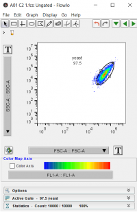 Protocol Figure 1
- Close the graph window and go back to the main workspace page and click on now gated “yeast” population below the first sample. This will open up a new graph with only the gated cells.
- We will now change our axis on the yeast scatterplot to analyze the data based on the fluorescence markers used in the secondary staining. Change the x-axis of the plot from “FSC-A::FSC-A” to “FL1-A::FL1-A” and the y-axis of the plot from “SSC-A::SSC-A” to “FL4-A::FL4-A”.
- The FL1-A channel and x-axis will measure the fluorescence intensity of the AF488 marker on our cells. Thus, dots farther to the right on the x axis represent cells that displayed more scFv on their surface.
- The FL4-A channel and y-axis will measure the fluorescence intensity of the AF647 marker on our cells. Thus, dots higher on the y axis represent cells with scFvs that bound lysozyme.
- We will now set two gates: yeast that displayed scFvs and yeast that did not display scFv. Despite the induction with galactose media not all yeast cells will display scFv on their surface (ex. Dead cells, budding cells). We want to analyze only the cells that displayed scFvs on their surface (right population) but we can use the non-displaying cell population (left population) to subtract the background fluorescence signal.
- Use the rectangle gating tool at the top to make a “displaying yeast” population and a “non-displaying yeast” population. Your plot should look like Figure 2 below:
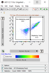 Protocol Figure 2
- Use the rectangle gating tool at the top to make a “displaying yeast” population and a “non-displaying yeast” population. Your plot should look like Figure 2 below:
- We will now add statistics to our graph to obtain the Median Fluorescence Intensity of the y-axis AF647 binding signal. Under the “Edit” tab, choose “Add a Statistic”. A pop-up menu will appear.
- Choose the “displaying yeast” as your population drop-down option.
- Choose “Median” in the statistic options menu on the left.
- Choose “FL4-A::FL4-A” as the statistic options menu on the left and select “Add” at the bottom.
- Repeat the above steps but now add the same statistic to the “non-displaying yeast” population
- Close the graph and return to the workspace screen. Your first sample should now have the following sub-populations listed below:
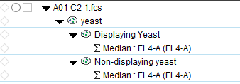 Protocol Figure 3
 - We now need to copy all of the sub-populations and statistics below the first sample to the other samples in our workspace. Select all of the subpopulations and statistics (select top, hold shift key, select bottom) and copy them (via ctrl+c, or copy in edit tab). Select the remaining samples and paste the subpopulations and statistics. All of the samples should now have the same five sub-populations and statistics.
- At this point, we need to check our control samples to ensure our gates are set correctly. The below image shows the three controls for Clone5, one sample with no staining, one sample with only AF488 staining, and one sample with only AF647 staining. The few errant dots in the AF647 control shows that yeast cells can sometimes be sticky to AF647 even without displaying scFv. We want to make sure that our "displaying yeast" gate excludes cells that do not display scFvs but may be slightly sticky to AF488. Fortunately, as you can see in the first two controls, we have set out gate to include minimal sticky cells.
- Next, we will export the statistics in a table. Under the “FlowJo” tab, select “Table Editor”
- Under the “Edit” tab in the Table Editor pop up window, select “Add Column”.
- Add the two statistics to your table that you just added to your samples in your workspace using the same populations (displaying and then non-displaying), statistics (Median), and parameter (FL4-A::FL4-A). Your window should look like the following:
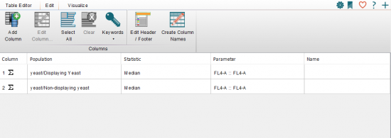 Protocol Figure 5
 - Return to the “Table Editor” tab and “Create Table” by pressing the gear symbol.
- Save the table as an excel file for further analysis.


In your laboratory notebook, complete the following:
Part 2: Plot titration binding curves via Matlab
Motivation:
You will also need to download the Matlab code from the 'Matlab Code' folder. You may chose to run Matlab on your computer, or by using the online Matlab server found here: Matlab Online. Please note that you will need to make an account with Matlab using your MIT email address and use the MIT software license for free access. Instructions below are for Matlab online.
- Open
In your laboratory notebook, complete the following:
- Report the Kd of each of the clones from your graph.
- Which scFv has the highest Kd?
- Which scFv has the lowest Kd?
- Rank the scFvs in order from weakest to strongest lysozyme binders.
Reagents list
Next day: Perform protein purification protocol