Difference between revisions of "Spring 2020 Assignment 8"
From Course Wiki
(→Convolution practice) |
Juliesutton (Talk | contribs) (→Fourier transform table) |
||
| (9 intermediate revisions by one user not shown) | |||
| Line 1: | Line 1: | ||
{{Template: 20.309}} | {{Template: 20.309}} | ||
| + | ==Circuit analogies== | ||
| + | {{Template:Assignment Turn In|message= | ||
| + | For each of the systems below, find an analogous circuit. | ||
| + | }} | ||
| + | |||
| + | <gallery> | ||
| + | File:Thermal System Analogy Problem.png |Thermal system:Coffee in a thermos | ||
| + | File:Mechanical System Analogy Problem.png|Mechanical system: mass and damper | ||
| + | </gallery> | ||
| + | |||
==Convolution practice== | ==Convolution practice== | ||
{{Template:Assignment Turn In|message= | {{Template:Assignment Turn In|message= | ||
| Line 6: | Line 16: | ||
{| style="width: 85%;" | {| style="width: 85%;" | ||
| − | !A | + | !<math>A</math> |
| − | !B | + | !<math>B</math> |
| − | !Y | + | !<math>Y=A*B</math> |
|- | |- | ||
|[[File:delta(t+1)+delta(t-1).png|250 px]] | |[[File:delta(t+1)+delta(t-1).png|250 px]] | ||
| Line 15: | Line 25: | ||
|- | |- | ||
|[[File:delta(t+1)+delta(t-1).png|250 px]] | |[[File:delta(t+1)+delta(t-1).png|250 px]] | ||
| − | |[[File:box w=1.png|250 px | + | |[[File:box w=1.png|250 px]] |
|[[File:bare convolution axes.png|250 px]] | |[[File:bare convolution axes.png|250 px]] | ||
|- | |- | ||
| Line 35: | Line 45: | ||
|} | |} | ||
| − | |||
| − | |||
| − | |||
| − | |||
| − | < | + | ==Fourier transform table== |
| − | + | The two tables below show important properties of the Fourier transform and several useful transform pairs. You can use the tables of pairs and properties to figure out the transforms of an endless number of functions. | |
| − | + | ||
| − | </ | + | {{Template:Assignment Turn In|message= |
| + | <ol type="A"> | ||
| + | <li>For each of the named functions in the ''Table of Common Functions and their Fourier Transforms'', sketch the function in the time domain as well as the magnitude of its Fourier transform. Show relevant constants (for example: ''a'', <math>\alpha</math>, and <math>f_0</math>).</li> | ||
| + | <li>Sketch the transform of <math>\cos^4(\omega_0 t)</math>.</li> | ||
| + | <li>Sketch the magnitude of the fourier transform of <math>e^{-\alpha t} u(t) \times \cos(\omega_0 t)</math>. Assume <math>\alpha\ll\omega_0</math>.</li> | ||
| + | }} | ||
| − | + | <center> | |
| + | [[Image: FourierTransformsTable.png|500 px|<caption>Short table of Fourier transform properties</caption>]] | ||
| + | [[Image: TimeFrequencyDomains_MoreTransformPairsTable.png|500 px|<caption>Short table of Fourier transform pairs</caption>]] | ||
| + | </center> | ||
| − | |||
{{Template: 20.309 bottom}} | {{Template: 20.309 bottom}} | ||
Latest revision as of 19:09, 27 April 2020

Circuit analogies
| |
For each of the systems below, find an analogous circuit. |
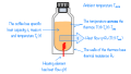
Thermal system:Coffee in a thermos
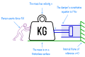
Mechanical system: mass and damper


Convolution practice
| |
For each of the pairs of functions below, plot the convolution of the two functions, $ Y=A*B $ |
| $ A $ | $ B $ | $ Y=A*B $ |
|---|---|---|
%2Bdelta(t-1).png)
|
|

|
|
|

|
|
|
|

|
|
|
|
|
|
|
|

|
|
.png)
|
|
|
Fourier transform table
The two tables below show important properties of the Fourier transform and several useful transform pairs. You can use the tables of pairs and properties to figure out the transforms of an endless number of functions.
| |
</div> |

